Readers can use IDLE, Spyder or a Jupyter notebook. The solutions here are shown in a Jupyter notebook.
$\bf{1.}$ Compute the following:
(a) $101-34+67$.
(b) $12 \times 7$.
(c) $4 \times (7 + 9 \times 3)$.
(d) $2-2 \times(2-4)$.
(e) $0.1 \div (0.6-0.05)$.
# 1(a) Addition and subtraction.
101 - 34 + 67
134
# 1(b) Use * for multiplication.
12 * 7
84
# 1(c)
4 * (7 + 9 * 3)
136
# 1(d)
2 - 2 * (2 - 4)
6
# 1(e) Use / for division.
0.1 / (0.6 - 0.05)
0.18181818181818185
$\bf{2.}$ Compute symbolically:
(a) $\frac{1}{4}-\frac{1}{5}$.
(b) $\frac{2}{3} \times 30$.
(c) $\frac{2}{5} \times \frac{5}{7}$.
(d) $\frac{1}{3} \div 2$.
(e) $\frac{1}{2} \times \left(\frac{1}{4} - \frac{1}{3} \right) \div \frac{1}{8}$.
# 2(a)
from fractions import Fraction
Fraction(1 , 4) - Fraction(1 , 5)
Fraction(1, 20)
# 2(b)
Fraction(2 , 3) * 30
Fraction(20, 1)
# 2(c)
Fraction(2 , 5) * Fraction(5 , 7)
Fraction(2, 7)
# 2(d)
Fraction(1 , 3) / 2
Fraction(1, 6)
# 2(e)
Fraction(1 , 2) * (Fraction(1 , 4) - Fraction(1 , 3)) / Fraction(1 , 8)
Fraction(-1, 3)
$\bf{3.}$ Determine:
(a) $2^{15}$.
(b) $\left( \frac{1}{3} \right)^3$.
(c) $64^{-2}$.
(d) $10^5 \times 10^{10}$.
(e) $\left(2^5\right)^3\left(\sqrt[3]{27} \times \sqrt[4]{625} - \sqrt[5]{32} \right)$.
# 3(a)
2**15
32768
# 3(b)
(Fraction(1 ,3))**3
Fraction(1, 27)
# 3(c)
Fraction(64 , 1)**(-2)
Fraction(1, 4096)
# 3(d)
10**5 * 10**10
1000000000000000
# 3(e)
from math import pow
(2**5)**3 * (pow(27 , 1 / 3) * pow(625 , 1 / 4) - pow(32 , 1 / 5))
425984.0
$\bf{4.}$ Read about all of the functions in the Math library. Use the Math library (module) to:
(a) Compute fmod$(36,5)$.
(b) Find the factorial, $52!$ and state how this number relates to a pack of playing cards?
(c) Find $\ln(2)$, where $\ln(x)=\log_e(x)$ is the natural logarithm function.
(d) Determine floor($\pi$) $-$ ceil(e).
(e) Compute the lowest common multiple of 6, 7 and 9.
# 4(a) The math modulo operation.
from math import *
fmod(36 , 5)
1.0
# 4(b)The number of permutations of a pack of cards.
factorial(52)
80658175170943878571660636856403766975289505440883277824000000000000
# 4(c) Natural logarithm.
log(2)
0.6931471805599453
# 4(d) The floor and ceiling functions.
floor(pi) - ceil(e)
0
# 4(e) Lowest common multiple.
lcm(6 , 7 , 9)
126
© Stephen Lynch 2023-present.
(Use IDLE, Spyder or a Jupyter notebook)
$\bf{1.}$ (a) Given the list, $A=[[1,2,3,4],[5,6,7,8],[9,10,11,12],[13,14,15,16]]$, how would you access the third element in the second list?
(b) Thinking of A as a 4x4 array, slice $A$ to remove row 3 and columns 1 and 2.
(c) Construct a list of the form: $[-9,-5,-1,\ldots,195,199]$.
(d) Create a dictionary data type for a car with key:value pairs, brand:BMW, year:2018, color:red, mileage:30000, and fuel:petrol.
# 1. (a) Accessing elements in lists of lists.
A = [[1,2,3,4] , [5,6,7,8] , [9,10,11,12] , [13,14,15,16]]
A[1][2]
7
# 1. (b) Slicing. Make up your own examples in order to understand.
[A[0][2:] , A[1][2:] , A[3][2:]]
[[3, 4], [7, 8], [15, 16]]
# 1. (c) Use range.
print(list(range(-9 , 200 , 4)))
[-9, -5, -1, 3, 7, 11, 15, 19, 23, 27, 31, 35, 39, 43, 47, 51, 55, 59, 63, 67, 71, 75, 79, 83, 87, 91, 95, 99, 103, 107, 111, 115, 119, 123, 127, 131, 135, 139, 143, 147, 151, 155, 159, 163, 167, 171, 175, 179, 183, 187, 191, 195, 199]
# 1. (d) Create a dictionary.
car = {"brand" : "BMW" , "year" : "2018" , "color" : "red" , "mileage" : "30000" , "fuel" : "petrol"}
$\bf{2.}$ Write a function for converting Kelvin to degrees Centigrade.
# 2. Kelvin to Centigrade.
def K2C():
    K = int(input('Enter temperature in Kelvin: '))
    C = K - 273.15
    # Format the output to four significant figures.
    print('Temperature in Centigrade is {:0.4g} degrees C'.format(C))
K2C()
Enter temperature in Kelvin: 0
Temperature in Centigrade is -273.1 degrees C
$\bf{3.}$ (a) Define a function called sigmoid whose formula is given by:
$$ \sigma(x)=\frac{1}{1+e^{-x}}, $$where $x$ is a real number. Determine $\sigma(0.5)$. This is an activation function used in AI.
(b) The function hsgn(x) is defined as:
$$ \mathrm{hsgn}(x)= \left \{ \begin{array} \\ 1 & \mathrm{if} & x > 0 \\ 0 & \mathrm{if} & x = 0 \\ -1 & \mathrm{if} & x < 0 \\ \end{array} \right . .$$Write a Python program that defines this function and determine $\mathrm{hsgn}(-6)$.
# 3. (a) Sigmoid function.
import numpy as np
def sigmoid(x):
    return 1 / (1 + np.exp(-x))
sigmoid(0.5)
0.6224593312018546
# 3. (b) hsgn function.
def hsgn(x):
    if x > 0:
        return 1
    elif x==0:
        return 0
    else:
        return -1
hsgn(-6)
-1
$\bf{4.}$ (a) Write an interactive Python program to play a “guess the number” game. The computer should think of a random integer between 1 and 20, and the user (player) has to try to guess the number within six attempts. The program should let the player know if the guess is too high or too low. Readers will need the randint function from the random module, examples and syntax can be found on the internet.
(b) Consider Pythagorean triples, positive integers $a,b,c$, such that $a^2 +b^2 = c^2$. Suppose that $c$ is defined by $c = b + n$, where $n$ is also an integer. Write a Python program that will find all such triples for a given value of $n$, where both $a$ and $b$ are less than or equal to a maximum value, $m$, say. For the case $n = 1$, find all triples with $1 \leq a \leq 100$ and $1 \leq b \leq 100$. For the case $n = 3$, find all triples with $1 \leq a \leq 200$ and $1 \leq b \leq 200$.
# 4. (a) Guess the number.
import random # Import the random module.
num_guesses = 0
name = input('Hi! What is your name? ')
number = random.randint(1, 20) # A random integer between 1 and 20.
print('Welcome, {}! I am thinking of an integer between 1 and 20.'.format(name))
while num_guesses < 6:
    guess = int(input('Take a guess and type the integer? '))
    num_guesses += 1
    if guess < number:
        print('Your guess is too low.')
    if guess > number:
        print('Your guess is too high.')
    if guess == number:
        break
if guess == number:
    print('Well done {}! You guessed my number in {} guesses!'.format(name, num_guesses))
else:
    print('Sorry, you lose! The number I was thinking of was {}'.format(number))
Hi! What is your name? Seb
Welcome, Seb! I am thinking of an integer between 1 and 20.
Take a guess and type the integer? 10
Your guess is too low.
Take a guess and type the integer? 15
Your guess is too low.
Take a guess and type the integer? 17
Your guess is too high.
Take a guess and type the integer? 16
Well done Seb! You guessed my number in 4 guesses!
# 4. (b) Pythagorean triples.
import math
def pythagorean_triples(i):
    for b in range(i):
        for a in range(1, b):
            c = math.sqrt( a * a + b * b)
            n = 1
            if c - b == n:
                print(a, b, int(c))
pythagorean_triples(101)
import math
def pythagorean_triples(i):
    for b in range(i):
        for a in range(1, b):
            c = math.sqrt( a * a + b * b)
            n = 3
            if c - b == n:
                print(a, b, int(c))
pythagorean_triples(201)
3 4 5
5 12 13
7 24 25
9 40 41
11 60 61
13 84 85
9 12 15
15 36 39
21 72 75
27 120 123
33 180 183
© Stephen Lynch 2023-present.
(Use Google Colab)
Plot a variation of the Cantor set, where the two middle third segments are removed at each stage. So at each stage, one segment is replaced with three segments each one-fifth the length of the previous segment.
Plot a Koch square fractal, where on each side of a square, one segment is replaced with five segments.
Plot a trifurcating tree.
Plot a Sierpinski square fractal, where at each stage a central square is removed and the length scales decrease by one third.
# You must run this cell before the other turtle programs.
# These commands are not needed in IDLE.
!pip install ColabTurtlePlus
from ColabTurtlePlus.Turtle import *
# 1. A variation of the Cantor set.
initializeTurtle()
def cantor3(x , y , length):
  speed(13)
  if length >= 1:
    penup()
    pensize(2)
    pencolor("blue")
    setpos(x , y)
    pendown()
    fd(length)
    y -= 80
    cantor3(x , y , length / 5)
    cantor3(x + 2 * length / 5 , y , length / 5)
    cantor3(x + 4 * length / 5 , y , length / 5)
    penup()
    setpos(x , y + 80)
cantor3(-300 , 200 , 600)
# 2. A Koch square fractal.
initializeTurtle()
pensize(1)
rt(90)
def KochSquare(length, level):
  speed(13)  # Fastest speed.
  for i in range(4):
    plot_side(length, level)
    rt(90)

def plot_side(length, level):
  if level==0:
    fd(length)
    return
  plot_side(length/3, level-1)
  lt(90)
  plot_side(length/3, level-1)
  rt(90)
  plot_side(length/3, level-1)
  rt(90)
  plot_side(length/3, level-1)
  lt(90)
  plot_side(length/3, level-1)
KochSquare(200 , 3)
# 3. A trifurcating tree.
initializeTurtle()
speed(13)
setheading(90)
penup()
setpos(0 , -200)
pendown()
def FractalTreeColor(length, level):
  pensize(length /10) # Thickness of lines.
  if length < 20:
    pencolor("green")
  else:
    pencolor("brown")
  if level > 0:
    fd(length)  # Forward
    rt(50)      # Right turn 50 degrees
    FractalTreeColor(length*0.7, level-1)
    lt(120)      # Left turn 120 degrees
    FractalTreeColor(length*0.5, level-1)
    rt(60)      # Right turn 60 degrees
    FractalTreeColor(length*0.5, level-1)
    rt(10)      # Right turn 10 degrees
    penup()
    bk(length)  # Backward
    pendown()
FractalTreeColor(200,6)
# 4. Sierpinski square.
initializeTurtle()
speed(13)
penup()
setpos(-200 , -200)
pendown()
def SierpinskiSquare(length, level):
  if level==0:
    return
  begin_fill() # Fill shape
  color("red")
  for i in range(4):
    SierpinskiSquare(length/3, level-1)
    fd(length/2)
    SierpinskiSquare(length/3, level-1)
    fd(length/1)
    lt(90) # Left turn 90 degrees
  end_fill()
SierpinskiSquare(200 , 3)
© Stephen Lynch 2023-present.
NumPy is a library that allows Python to compute with lists, arrays, vectors, matrices and tensors:
https://numpy.org/doc/stable/reference/
Matplotlib is an acronym for MATrix PLOTting LIBrary and it is a comprehensive library for creating animated, static, and more recently, interactive visualizations in Python. For more information the reader is directed to the URL:
${\bf 1.}$ Plot the graph of the quadratic function: $y=f(x)=x^2-3x-18$.
${\bf 2.}$ Plot the graph of the trigonometric function: $y=g(x)=2+3 \sin(x)$.
${\bf 3.}$ Plot the graph of the exponential function: $y=h(x)=1 + e^{-x}$.
${\bf 4.}$ Plot the three-dimensional surface: $z=xe^{-\left( x^2+y^2 \right)}$.
# 1. Plot a parabola.
import numpy as np
import matplotlib.pyplot as plt
x = np.linspace(-5 , 8 , 100)     # Define the domain values.
y = x**2 - 3 * x -18              # A vector of y-values.
plt.plot(x , y)
plt.title("$y=f(x)=x^2-3x-18$")
plt.xlabel("x")
plt.ylabel("y")
plt.show()

# 2. Plot a trigonometric function.
# Simple plots in Python.
import numpy as np
import matplotlib.pyplot as plt
x = np.linspace(-2 * np.pi , 2 * np.pi , 100)  # Define the domain values.
y = 2 + 3 * np.sin(x)                          # A vector of y-values.
plt.axis([-2 * np.pi , 2 * np.pi , -2 , 6])    # Set the range of x and y-values.
plt.plot(x , y)
plt.title("$y=g(x)=2+3\sin(x)$")
plt.xlabel("x")
plt.ylabel("y")
plt.show()

# 3. Plot an exponential function.
# Simple plots in Python.
import numpy as np
import matplotlib.pyplot as plt
x = np.linspace(-2 , 8 , 100)  # Define the domain values.
y = 1 + np.exp(-x)             # A vector of y-values.
plt.plot(x , y)
plt.title("$y=h(x)=1+e^{-x}$")
plt.xlabel("x")
plt.ylabel("y")
plt.show()

# 4. Plotting a surface in 3D.
# You can rotate the figure. Un-comment the line below.
# %matplotlib qt5 - Un-comment: An interactive window will appear in this case.
from mpl_toolkits.mplot3d import axes3d
import matplotlib.pyplot as plt
import numpy as np
x = np.arange(-2 , 2 , 0.1)
y = np.arange(-2 , 2 , 0.1)
X,Y = np.meshgrid(x,y)
# Z is a function of two variables.
Z = X * np.exp(-X**2 - Y**2)
fig = plt.figure(figsize=(12,6))
ax = fig.add_subplot(111, projection = "3d")
ax.set_xlabel("x")
ax.set_ylabel("y")
ax.set_zlabel("z")
ax.set_zlim(np.min(Z) , np.max(Z))
ax.set_title("3D Surface, $z=xe^{-x^2-y^2}$")
ax.plot_surface(X , Y , Z)
plt.show()

© Stephen Lynch 2023-present.
Create your own notebook and include the questions in your solutions.
${\bf 1.}$ Use SymPy to:
(a) Factorize $x^3-y^3$.
(b) Solve $x^2-7x-30=0$.
(c) Split into partial fractions $\frac{3x}{(x-1)(x+2)(x-5)}$.
(d) Expand $(y+x-3)(x^2-y+4)$.
(e) Solve the linear simultaneous equations: $y=2x+2$ and $y=-3x+1$.
SymPy is a computer algebra system and a Python library for symbolic mathematics written entirely in Python. For more information, see the sympy help pages at:
# Import all of the functions from the SymPy library.
from sympy import *
x , y = symbols("x y") # Declare symbolic objects.
# 1. (a) Factorization.
factor(x**3 - y**3)
# 1. (b) Solve the algebraic quadratic equation.
solve(x**2 - 7 * x - 30 , x)
[-3, 10]
# 1. (c) Partial fractions.
apart(3 * x / ((x - 1) * (x + 2) * (x - 5)))
# 1. (d) Expansion.
expand((x + y - 3) * (x**2 - y + 4))
# 1. (e) Solving linear simultaneous equations.
solve([2 * x + 2 - y , y + 3 * x - 1] , [x , y])
{x: -1/5, y: 8/5}
${\bf 2.}$ Compute the following using SymPy:
(a) $\lim_{x \rightarrow 1} \frac{x-1}{x^2-1}$.
(b) The dervivative of $y=x^2-6x+9$.
(c) The derivative of $y=\cos(3x)$.
(d) The derivative of $y=2e^x-1$.
(e) The derivative of $y=x\sin(x)$.
# 2. (a) Limits.
limit((x - 1) / (x**2 - 1) , x , 1)
# 2. (b) Differentiation.
diff(x**2 - 6 * x + 9 , x)
# 2. (c) Differentiation.
diff(cos(3 * x) , x)
# 2. (d) Differentiation.
diff(2 * exp(x) - 1 , x)
# 2. (e) Differentiation.
diff(x * sin(x) , x)
${\bf 3.}$ Determine the following integrals using SymPy:
(a) $\int x^5 dx$.
(b) $\int_{x=1}^{4} x^5dx$.
(c) $\int \cos(3x) dx$.
(d) $\int_{x=0}^{1} x\sin(x)dx$.
(e) $\int_{x=1}^{\infty} \frac{1}{x}dx$. Use oo for $\infty$ in Python.
# 3. (a) Indefinite integration.
print(integrate(x**5) , "+ c")
x**6/6 + c
# 3. (b) Definite integration (to determine the area under a curve).
integrate(x**5 , (x , 1 , 4))
# 3. (c) Indefinite integration.
print(integrate(cos(3 * x) , x) , "+ c")
sin(3*x)/3 + c
# 3. (d) Definite integration (to determine the area under a curve).
integrate(x * sin(x) , (x , 0 , 1))
# 3. (e) Improper integration (to determine the area under a curve).
integrate(1 / x , (x , 1 , oo))
${\bf 4.}$ Given that
$A=\begin{pmatrix} 1 & 2 \\ -1 & 0 \end{pmatrix}$ and $B=\begin{pmatrix} 1 & -3 \\ 4 & 7 \end{pmatrix}$,
determine:
(a) $2A$.
(b) $3A+4B$.
(c) $A \times B$.
(d) The inverse of $A$, if it exists.
(e) The determinant of $B$.
# 4. (a) Define two 2x2 matrices.
A , B = Matrix([[1 , 1] , [-1 , 0]]) , Matrix([[1 , -3] , [4 , 7]])
2 * A
# 4 (b). Matrix algebra.
3 * A + 4 * B
# 4 (c). Multiplying matrices.
A * B
# 4 (d). Matrix inverse.
A.inv()
# 4 (e). The determinant.
B.det()
${\bf 5.}$ Sign up to GitHub and upload your notebooks to your repository.
GitHub is a website and cloud-based service that helps developers store and manage their code, as well as track and control changes to their code.
To sign up to GitHub, where the world builds software, click here:
Upload this Google Colab notebook to GitHub.
DID YOU KNOW? You can use GitHub to host your own web pages.
© Stephen Lynch 2023-present.
$\bf{ 1.}$ (a) Given $s=ut+\frac{1}{2}at^2$, determine $s$ if $u=1$, $t=1$, and $a=9.8$.
(b) Expand $2x(x-4)$.
(c) Expand $(x+y+1)(x-y+2)$.
(d) Factorize $x^2-7x+12$.
# 1. (a) Substitution.
u , t , a = 1 , 1 , 9.8
s = u * t + a * t**2 / 2
print("s = " , s)
s = 5.9
# 1. (b) Expansion.
from sympy import symbols , expand
x , y = symbols("x  y")
expand(2 * x * (x - 4))
# 1. (c) Expansion.
expand((x + y + 1) * (x - y + 2))
# 1. (d) Factorization.
from sympy import factor
factor(x**2 - 7 * x + 12)
$\bf{ 2.}$ (a) Solve for $t$ given, $3=5+10t$.
(b) Solve for $a$ given, $s=ut+\frac{1}{2}at^2$.
(c) Solve the quadratic equation, $2x^2+x-3=0$.
(d) Determine where the line $y=x$ meets the circle $x^2+y^2=1$.
# 2. (a) Solve for t.
from sympy import symbols, solve
t = symbols("t")
solve(3 -5 - 10 * t , t)
[-1/5]
# 2. (b) Solve for a.
a , s , u , t = symbols("a s u t")
solve(s - u * t - a * t**2 / 2 , a)
[2*(s - t*u)/t**2]
# 2. (c) Solve for x.
x = symbols("x")
solve(2 * x**2 + x - 3 , x)
[-3/2, 1]
# 2. (d) Where a line meets a circle.
sol = solve([y - x , x**2 + y**2 - 1] , [x , y])
print(sol)
[(-sqrt(2)/2, -sqrt(2)/2), (sqrt(2)/2, sqrt(2)/2)]
$\bf{ 3.}$ (a) If $f(x)=\frac{2x+3}{x-5}$, determine $f(4)$.
(b) Plot the function $f(x)=\frac{2x+3}{x-5}$, and determine where $f(x)=1$.
(c) Given $g(x)=3x+4$ and $h(x)=1-x^2$, find $g(h(x))-h(g(x))$.
(d) The logistic map function is defined by, $f_{\mu}(x)=\mu x(1-x)$. Compute $f_{\mu}\left(f_{\mu}(x) \right)$.
# 3. (a) Define a function.
def f(x):
    return (2 * x + 3) / (x - 5)
print("f(4) = " , f(4))
f(4) = -11.0
# 3. (b) Define a function and determine when it is equal to one.
import matplotlib.pyplot as plt
import numpy as np
from sympy import *
def g(x):
    return (2 * x + 3) / (x - 5)
x = np.linspace(-10 , 10 , 100)
y = (2 * x + 3) / (x - 5)
plt.xlabel("x")
plt.ylabel("f(x)")
plt.plot(x , y)
plt.ylim(-50 , 50)
plt.show()
x = symbols("x")
sol = solve((2 * x + 3) / (x - 5) - 1 , x)
print("y=f(x)=1, when " , "x =" , sol[0])

y=f(x)=1, when x = -8
# 3. (c) Functions of functions (composition of functions).
def g(x):
    return 3 * x + 4
def h(x):
    return 1 - x**2
print("g(h(x))-h(g(x)) = " , g(h(x)) - h(g(x)))
g(h(x))-h(g(x)) = -3*x**2 + (3*x + 4)**2 + 6
# 3. (d) Functions of functions (composition of functions).
mu = symbols("mu")
def f_mu(x):
    return mu * x * (1 - x)
print("f_mu(f_mu(x)) = " , f_mu(f_mu(x)))
f_mu(f_mu(x)) = mu**2*x*(1 - x)*(-mu*x*(1 - x) + 1)
$\bf{ 4.}$ (a) If $y=\sin(2x)$, compute $\frac{dy}{dx}$.
(b) Determine $\left. \frac{dy}{dx} \right|_{x=0}$ for $y=x^3-1$.
(c) Determine the area bound by the curves, $y=1-x^2$ and $y=x^2-1$.
(d) Plot the curves, $y=1-x^2$ and $y=x^2-1$, and shade the area between the curves.
# 4. (a) Differentiate
from sympy import *
x , y = symbols("x y")
print("dy/dx = " , diff(sin(2 * x) , x))
dy/dx = 2*cos(2*x)
# 4. (b) Find the gradient at x=0. Use the subs function from sympy.
x , y , c = symbols("x y c")
xval = 0
y = x**3 - 1
dydx = diff(y , x)
# The gradient (m) of the tangent.
m = dydx.subs(x , xval)
print("m = " , m)
m = 0
# 4. (c) Using integration to determine the area.
# Determine where the graphs meet.
soln = solve([1 - x**2 , x**2 - 1])
A = integrate((1 - x**2) - (x**2 - 1) , (x , soln[0].get(x) , soln[1].get(x)))
print("Area = " , A , "units squared")
Area = 8/3 units squared
# 4. (d) Shading the area between the curves.
import numpy as np
from matplotlib import pyplot as plt
def f(x):
    return 1 - x**2
def g(x):
    return x**2 - 1
x = np.arange(-1.2 , 1.2 , 0.01)
plt.plot(x , f(x) , x , g(x))

# Shade the area.
plt.fill_between(
        x = x,
        y1 = f(x),
        y2 = g(x),
        where = (-1 <= x) & (x <= 1),  # Limits of integration.
        color = "b",                   # Color of shading.
        alpha = 0.3)                   # Transparency.
plt.show()

A Jupyter notebook showing how you can use Python to give a deeper understanding of A-Level (High-School) Maths:
https://drstephenlynch.github.io/webpages/Python_for_A_Level_Mathematics_and_Beyond.html
The notebook covers all of the material in the UK A-Level Mathematics syllabus.
Students get a deeper understanding by checking handwritten results, plotting curves and producing animations.
© Stephen Lynch 2023-present.
$\bf{ 1.}$ Write a Python program to decrypt a Caesar cipher.
Caesar's cipher is one of the simplest encryption techniques and is often used by children when learning how to send secret messages. It is a type of substitution cipher in which each letter in the plaintext is replaced by a letter some fixed number of positions down the alphabet.
Wikipedia: https://en.wikipedia.org/wiki/Caesar_cipher
Unicode is a universal character encoding standard.
List of Unicode Characters: https://en.wikipedia.org/wiki/List_of_Unicode_characters
# 1. The Caeser Cipher: Decryption.
shift = 3
def decrypt(text , shift):
    result = ""
    for i in range(len(text)):
        char = text[i]
        if (char.isupper()): # Upper-case characters.
            result += chr((ord(char) - shift - 65) % 26 + 65)
        else:                # Lower-case characters.
            result += chr((ord(char) - shift - 97) % 26 + 97)
    return result

# Insert text.
text = "FdhvhuqFlskhuqFrgh"
print("Text : " + text)
print("Shift : " + str(shift))
print("Cipher: " + decrypt(text,shift))
Text : FdhvhuqFlskhuqFrgh
Shift : 3
Cipher: CaesernCiphernCode
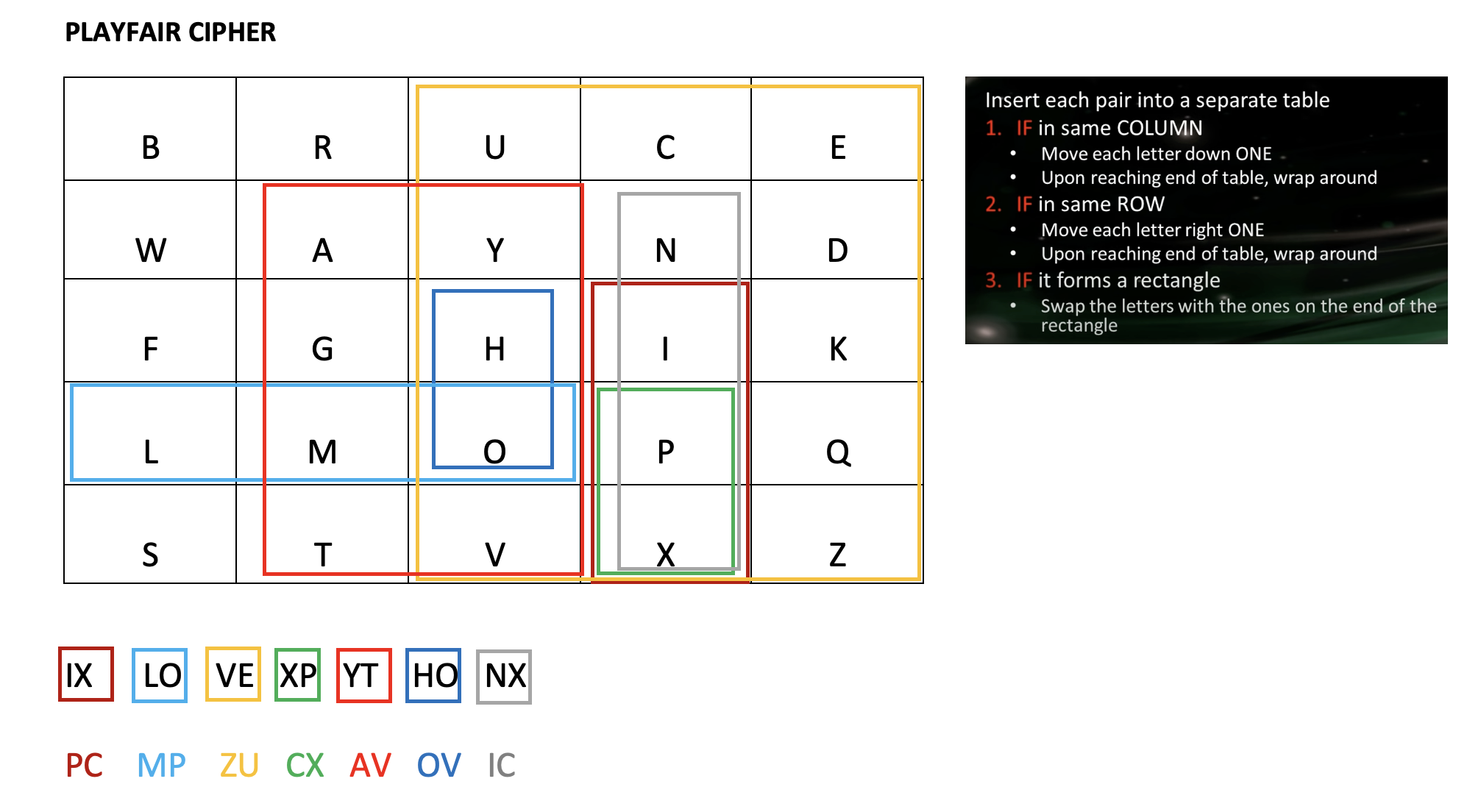
Matrix =$\begin{pmatrix} B & R & U & C & E \\ W & A & Y & N & D \\ F & G & H & I & K \\ L & M & O & P & Q \\ S & T & V & X & Z \end{pmatrix}$
$\bf{ 3.}$ The Vigenère cipher, first described by Giovan Battista Bellaso in 1553, is a method of encrypting alphabetic text where each letter of the plaintext is encoded with a different Caesar cipher, whose increment is determined by the corresponding letter of another text, the key. Write a Python program for the Vigenère cipher:
# 3. Vigenere Cipher Encryption.
def vigenere(key, message):
    message = message.lower()
    # message = message.replace(" ","")
    key_length = len(key)
    cipher_text = ""
    for i in range(len(message)):
        letter = message[i]
        k = key[i % key_length]
        cipher_text = cipher_text + chr ((ord(letter) - 97 + k ) % 26 + 97)
    return cipher_text

if __name__=="__main__":
    print ("Encryption")
    key = "rosebud"
    key = [ord(letter)-97 for letter in key]

    cipher_text = vigenere(key , "Vigenere Cipher")
    print ("cipher text: ",cipher_text)
Encryption
cipher text:  mwyioyuvbumqbhi
$\bf{ 4.}$ For those interetsed in cryptography, carry out a literature search on:
(a) Symmetric Cryptography: block ciphers, stream ciphers, hash functions, keyed hashing and authenticated encryption.
(b) Asymmetric Cryptography: Rivest-Shamir-Adleman (RSA) a public-key cryptosystem, Diffie-Hellman key exchange, authenticated encryption, elliptic curve cryptography and chaos synchronization cryptography.
(c) For this problem, use the RSA public key cryptosystem. Bob chooses the prime numbers $p=19$ and $q=23$ and $e=7$. Alice wishes to send the number 11 to Bob. What is the message sent? Confirm that Bob correctly decrypts this.
# 4. (c) RSA Public Key Cryptosystem.
# Check two numbers, p and q, are prime.
# In practice much larger primes would be chosen.
from sympy import *
isprime(19) , isprime(23)
(True, True)
# RSA Algorithm Example.
from math import gcd

# Step 1, choose two prime numbers (not large for this simple example).
p , q = 19 , 23

# Step 2, compute n.
n = p * q
print("n =", n)

# Step 3, compute phi(n).
phi = (p - 1) * (q - 1)

# Step 4, compute a public key, e say, there are many possibilities.
# In this case, choose e = 7.

#for e in range(2 , phi):
#    if (gcd(e, phi) == 1):
#        print("e =", e)
e = 7

# Step 5:
# Python program for the EEA.
def extended_gcd(e, phi):
    if e == 0:
        return phi, 0, 1
    else:
        gcd, x, y = extended_gcd(phi % e, e)
        return gcd, y - (phi // e) * x, x
if __name__ == '__main__':
    gcd, x, y = extended_gcd(e, phi)
    print("phi = " , phi)
    print('The gcd is', gcd)
    print("x = " , x , ", y = " , y)
n = 437
phi =  396
The gcd is 1
x =  -113 , y =  2
In order to encrypt and decrypt, one has to compute $x^y$mod$(z)$. In Python, we use the built-in function pow(x , y , z), which takes three arguments.
${\bf IMPORTANT:}$ If you import pow from the math library it only takes two arguments.
# Encryption and decryption.
# The message here is m = msg = 11.

d , e , n = -113 , 7 , 437
msg = 11
print(f"Original message: {msg}")

# Encryption
E = pow(msg , e , n)
print(f"Encrypted message: {E}")

# Decryption
D = pow(E , d , n)
print(f"Decrypted message: {D}")
Original message: 11
Encrypted message: 30
Decrypted message: 11
© Stephen Lynch 2023-present.
${\bf 1.}$ Given the activation functions:
$$\sigma(v)=\frac{1}{1+e^{-v}},$$$$\phi(v)=\tanh(v)=\frac{e^v-e^{-v}}{e^v+e^{-v}},$$show that:
(a) $\frac{d\sigma}{dv}=\sigma(v)(1-\sigma(v));$
(b) $\frac{d\phi}{dv}=1-(\phi(v))^2.$
Plot the curves and their derivatives.
# 1.(a)
from sympy import *
x = symbols("x")
sigmoid = 1 / (1 + exp(-x))
dsigmoid = diff(sigmoid , x)
simplify(dsigmoid - sigmoid * (1 - sigmoid))
# 1.(b)
from sympy import *
tanh = tanh(x)
dtanh = diff(tanh , x)
simplify(dtanh - (1 - tanh**2))
# 1: Activation functions and their derivatives.
import numpy as np
import matplotlib.pyplot as plt
x = np.linspace(-10, 10, 1000)
y = np.maximum(0, x)
plt.figure(figsize=(15, 10))
plt.subplot(1, 2, 1)
y = 1 / (1 + np.exp(-x) )
plt.plot(x, y,label = r"$\sigma(v)=\frac{1}{1+e^{-v}}$")
plt.plot(x, y * (1 - y), label = r"$\frac{d \sigma}{dv} = \sigma(v) (1 - \sigma(v))$" )
plt.xlabel("v")
plt.legend()

plt.subplot(1, 2, 2)
y = ( 2 / (1 + np.exp(-2*x) ) ) -1
plt.plot(x,y,label = r"$\phi(v)=\tanh(v)$")
plt.plot(x, 1 - y**2, label = r"$\frac{d \phi}{dv}=1 - \tanh^2(v)$")
plt.xlabel("v")
plt.legend()
plt.show()

${\bf 2.}$ Show that the XOR Gate ANN shown above acts as a good approximation of an XOR gate, given that:
$$w_{11}=60, w_{12}=80, w_{21} =60, w_{22} =80, w_{13} =−60, w_{23}=60,$$$$b_1 = −90, b_2 = −40, b_3=-30.$$Use the sigmoid transfer function in your program.
# 2: ANN for an XOR Logic Gate.
import numpy as np
w11 , w12 , w21 , w22 , w13 , w23 = 60 , 80 , 60 , 80 , -60 , 60
b1 , b2 , b3 = -90 , -40 , -30
def sigmoid(x):
  return 1 / (1 + np.exp(-x))

def XOR(x1 , x2):
  h1 = x1 * w11 + x2 * w21 + b1
  h2 = x1 * w12 + x2 * w22 + b2
  o1 = sigmoid(h1) * w13 + sigmoid(h2) * w23 + b3
  return sigmoid(o1)
print("XOR(0,0)= " , XOR(0 ,0))
print("XOR(0,1)= " , XOR(0 ,1))
print("XOR(1,0)= " , XOR(1 ,0))
print("XOR(1,1)= " , XOR(1 ,1))
XOR(0,0)=  9.357622968839299e-14
XOR(0,1)=  0.9999999999999065
XOR(1,0)=  0.9999999999999065
XOR(1,1)=  9.357622968891759e-14
${\bf 3.}$ Use backpropagation to update the weights $w_{11}, w_{12}, w_{21}$ and $w_{22}$ for the XOR Gate ANN in Example 8.2.1.
# 3: Backpropagation, keep the biases constant in this case.
import numpy as np
w11,w12,w21,w22,w13,w23 = 0.2,0.15,0.25,0.3,0.15,0.1
b1 , b2 , b3 = -1 , -1 , -1
yt , eta = 0 , 0.1
x1 , x2 = 1 , 1
def sigmoid(v):
    return 1 / (1 + np.exp(- v))
h1 = x1 * w11 + x2 * w21 + b1
h2 = x1 * w12 + x2 * w22 + b2
o1 = sigmoid(h1) * w13 + sigmoid(h2) * w23 + b3
y = sigmoid(o1)
print("y = ", y)
# Backpropagate.
dErrdw13=(yt-y)*sigmoid(o1)*(1-sigmoid(o1))*sigmoid(h1)
w13 = w13 - eta * dErrdw13
print("w13_new = ", w13)
dErrdw23=(yt-y)*sigmoid(o1)*(1-sigmoid(o1))*sigmoid(h2)
w23 = w23 - eta * dErrdw23
print("w23_new = ", w23)
dErrdw11=(yt-y)*sigmoid(o1)*(1-sigmoid(o1))*w13*sigmoid(h1)*(1-sigmoid(h1))*x1
w11 = w11 - eta * dErrdw11
print("w11_new = ", w11)
dErrdw12=(yt-y)*sigmoid(o1)*(1-sigmoid(o1))*w23*sigmoid(h2)*(1-sigmoid(h2))*x1
w12 = w12 - eta * dErrdw12
print("w12_new = ", w12)
dErrdw21=(yt-y)*sigmoid(o1)*(1-sigmoid(o1))*w13*sigmoid(h1)*(1-sigmoid(h1))*x2
w21 = w21 - eta * dErrdw21
print("w21_new = ", w21)
dErrdw22=(yt-y)*sigmoid(o1)*(1-sigmoid(o1))*w23*sigmoid(h1)*(1-sigmoid(h1))*x2
w22 = w22 - eta * dErrdw22
print("w22_new = ", w22)
y =  0.28729994077761756
w13_new =  0.1521522763401024
w23_new =  0.10215227634010242
w11_new =  0.20020766275648338
w12_new =  0.15013942100503588
w21_new =  0.2502076627564834
w22_new =  0.3001394210050359
${\bf 4.}$ Download the notebook: "Boston-Housing-ANN-Calculator.ipynb" from GitHib. Three attributes are used in the program (average number of rooms, index of accessible radial highways, percentage lower status of population). The target data is median value of owner-occupied homes. List 10 attributes which would be important to you when purchasing your house.
# 4: Backpropagation of errors - using the perceptron.
# Training Boston housing data (housing.txt).
# The target is the value of a house (column 13).
# In this case, use 3 attributes (columns 5, 8, and 12).

import matplotlib.pyplot as plt
import numpy as np

data = np.loadtxt('housing.txt')
rows, columns = data.shape
columns = 4  # Using 4 columns from the data in this case.

X = data[:, [5, 8, 12]]             # The three data coumns.
t = data[:, 13]                     # The target data.
ws1, ws2, ws3, ws4 = [], [], [], [] # Empty lists of weights.
k = 0

xmean = X.mean(axis=0)              # Normalize the data.
xstd = X.std(axis=0)
ones = np.array([np.ones(rows)])
X = (X - xmean * ones.T) / (xstd * ones.T)
X = np.c_[np.ones(rows), X]
tmean = (max(t) + min(t)) / 2
tstd = (max(t) - min(t)) / 2
t = (t - tmean) / tstd

w = 0.1 * np.random.random(columns)  # Set random weights.
y1 = np.tanh(X.dot(w))
e1 = t - y1
mse = np.var(e1)

num_epochs = 10  # Number of iterations is 506*num_epochs.
eta = 0.001      # The learning rate.
k = 1

# Backpropagation.
for m in range(num_epochs):
    for n in range(rows):
        yk = np.tanh(X[n, :].dot(w))
        err = yk - t[n]
        g = X[n, :].T * ((1 - yk**2) * err)
        w = w - eta*g
        k += 1
        ws1.append([k, np.array(w[0]).tolist()])
        ws2.append([k, np.array(w[1]).tolist()])
        ws3.append([k, np.array(w[2]).tolist()])
        ws4.append([k, np.array(w[3]).tolist()])

ws1 = np.array(ws1)
ws2 = np.array(ws2)
ws3 = np.array(ws3)
ws4 = np.array(ws4)

plt.plot(ws1[:, 0], ws1[:, 1], 'k', markersize=0.1,label = r"$b$")
plt.plot(ws2[:, 0], ws2[:, 1], 'g', markersize=0.1,label = r"$w_1$")
plt.plot(ws3[:, 0], ws3[:, 1], 'b', markersize=0.1,label = r"$w_2$")
plt.plot(ws4[:, 0], ws4[:, 1], 'r', markersize=0.1,label = r"$w_3$")
plt.xlabel('Number of iterations', fontsize=15)
plt.ylabel('Weights', fontsize=15)
plt.tick_params(labelsize=15)
plt.legend()
plt.show()

Once the weights have converged, the ANN can be used to value other homes. REMINDER: The data is from the 1970s.
Change the learning rate and number of epochs to see how the convergence is affected.
© Stephen Lynch 2023-present.
${\bf 1.}$ For the data set Data-1-OCR.xlsx, create a scatter plot of life expectancy against GDP, where the size of the filled circles is determined by physician density. What can you conclude?
# Load the data file and create a DataFrame.
import pandas as pd    # Import pandas for data analysis
import seaborn as sns  # Import seaborn for visualisations
import matplotlib.pyplot as plt
df1 = pd.read_excel("Data-1-OCR.xlsx" , sheet_name = "Data")
df1.head()
| no | Country | Region | population | birth rate per 1000 | death rate per 1000 | median age | labor force | unemployment (%) | GDP per capita (US$) | physician density (physicians/1000 population) | Health expenditure (% of GDP) | Total area | Land borders | Life expectancy at birth 1960 | Life expectancy at birth 1970 | Life expectancy at birth 1980 | Life expectancy at birth 1990 | Life expectancy at birth 2000 | Life expectancy at birth 2010 | |
|---|---|---|---|---|---|---|---|---|---|---|---|---|---|---|---|---|---|---|---|---|
| 0 | 1 | Algeria | Africa, N | 41657488 | 21.5 | 4.3 | 28.3 | 11820000.0 | 11.7 | 15200.0 | 1.83 | 7.2 | 2381740.0 | Yes | 46.138 | 50.369 | 58.196 | 66.725 | 70.292 | 74.676 |
| 1 | 2 | Egypt | Africa, N | 99413317 | 28.8 | 4.5 | 23.9 | 29950000.0 | 12.2 | 12700.0 | 0.79 | 5.6 | 1001450.0 | Yes | 48.056 | 52.155 | 58.338 | 64.580 | 68.613 | 70.357 |
| 2 | 3 | Libya | Africa, N | 6754507 | 17.2 | 3.7 | 29.4 | 1114000.0 | 30.0 | 9600.0 | 2.16 | 5.0 | 1759540.0 | Yes | 42.609 | 56.052 | 64.185 | 68.522 | 70.473 | 71.643 |
| 3 | 4 | Morocco | Africa, N | 34314130 | 17.5 | 4.9 | 29.7 | 12000000.0 | 10.2 | 8600.0 | 0.73 | 5.9 | 446550.0 | Yes | 48.458 | 52.572 | 57.560 | 64.733 | 68.722 | 73.999 |
| 4 | 5 | Sudan | Africa, N | 43120843 | 34.2 | 6.7 | 17.9 | 11920000.0 | 19.6 | 4300.0 | 0.41 | 8.4 | 1861484.0 | Yes | 48.194 | 52.234 | 54.253 | 55.500 | 58.430 | 62.620 |
# Create a scatter plot of life expectancy against GDP, where the size
# is determined by physicians per 1000.
# Sizes=(30 , 150) sets the range of sizes to be used.
sns.relplot(data=df1, x="GDP per capita (US$)", y="Life expectancy at birth 2010", size="physician density \
(physicians/1000 population)", sizes=(30, 150), aspect=2)
<seaborn.axisgrid.FacetGrid at 0x7fb393de0640>

Communicate the Results: When the physician density is low and the GDP per capita is also low, there is a low life expectancy at birth.
${\bf 2.}$ Load the data file, Data-2-Edexcel.xlsx from GitHub. This LDS consists of weather data samples provided by the UK Met Office for five UK weather stations. Load the data and set up a data frame. Explore the data. Plot box and whisker plots for Daily Mean Temperature for each station and compare the results in 2015 to 1987. Communicate the results.
import pandas as pd    # Import pandas for data analysis
import seaborn as sns  # Import seaborn for visualisations
import matplotlib.pyplot as plt
df2 = pd.read_csv("Data-2-Edexcel.csv")
df2.head()
| Date | Daily Mean Temperature | Daily Total Rainfall | Daily Total Sunshine | Daily Mean Windspeed | Daily Mean Windspeed (Beaufort) | Daily Maximum Gust | Daily Maximum Relative Humidity | Daily Mean Total Cloud | Daily Mean Visibility | Daily Mean Pressure | Daily Mean Wind Direction | Mean Cardinal Direction | Daily Max Gust Direction | Max Cardinal Direction | Station | Year | |
|---|---|---|---|---|---|---|---|---|---|---|---|---|---|---|---|---|---|
| 0 | 01/05/1987 | 10.7 | 3.1 | NaN | NaN | NaN | NaN | 100 | 7 | 2000 | 1018 | 360 | N | 20.0 | NNE | Camborne | 1987 |
| 1 | 02/05/1987 | 8.9 | 0.1 | NaN | NaN | NaN | NaN | 91 | 3 | 3200 | 1020 | 320 | NW | 330.0 | NNW | Camborne | 1987 |
| 2 | 03/05/1987 | 8.1 | 0 | NaN | NaN | NaN | NaN | 77 | 5 | 3600 | 1029 | 350 | N | 350.0 | N | Camborne | 1987 |
| 3 | 04/05/1987 | 8.2 | 0 | NaN | NaN | NaN | NaN | 83 | 5 | 4100 | 1036 | 350 | N | 350.0 | N | Camborne | 1987 |
| 4 | 05/05/1987 | 9.8 | 0 | NaN | NaN | NaN | NaN | 86 | 5 | 2700 | 1036 | 10 | N | 10.0 | N | Camborne | 1987 |
# Pre-process and clean the data.
# Create a new column called Rainfall which is a copy of the Daily Total Rainfall column.
df2["Rainfall"] = df2["Daily Total Rainfall"]
# Replace any instances of 'tr' with 0.025 and change the type to float.
df2["Rainfall"] = df2["Rainfall"].replace({"tr": 0.025}).astype("float")
df2.iloc[0 : 5 , 12 : 19]
| Mean Cardinal Direction | Daily Max Gust Direction | Max Cardinal Direction | Station | Year | Rainfall | |
|---|---|---|---|---|---|---|
| 0 | N | 20.0 | NNE | Camborne | 1987 | 3.1 |
| 1 | NW | 330.0 | NNW | Camborne | 1987 | 0.1 |
| 2 | N | 350.0 | N | Camborne | 1987 | 0.0 |
| 3 | N | 350.0 | N | Camborne | 1987 | 0.0 |
| 4 | N | 10.0 | N | Camborne | 1987 | 0.0 |
# Change the data type of a feature.
df2["Year"] = df2["Year"].astype("category")
df2.info()
# Create a box plot with a category on the y-axis, colour-coded by
# another category.
sns.catplot(data=df2, kind="box", x="Daily Mean Temperature",y="Station", hue="Year", \
            aspect=2)
plt.show()
<class 'pandas.core.frame.DataFrame'>
RangeIndex: 1840 entries, 0 to 1839
Data columns (total 18 columns):
 #   Column                           Non-Null Count  Dtype
---  ------                           --------------  -----
 0   Date                             1840 non-null   object
 1   Daily Mean Temperature           1840 non-null   float64
 2   Daily Total Rainfall             1840 non-null   object
 3   Daily Total Sunshine             1759 non-null   float64
 4   Daily Mean Windspeed             1757 non-null   float64
 5   Daily Mean Windspeed (Beaufort)  1757 non-null   object
 6   Daily Maximum Gust               1684 non-null   float64
 7   Daily Maximum Relative Humidity  1840 non-null   int64
 8   Daily Mean Total Cloud           1840 non-null   int64
 9   Daily Mean Visibility            1840 non-null   int64
 10  Daily Mean Pressure              1840 non-null   int64
 11  Daily Mean Wind Direction        1840 non-null   int64
 12  Mean Cardinal Direction          1840 non-null   object
 13  Daily Max Gust Direction         1832 non-null   float64
 14  Max Cardinal Direction           1832 non-null   object
 15  Station                          1840 non-null   object
 16  Year                             1840 non-null   category
 17  Rainfall                         1840 non-null   float64
dtypes: category(1), float64(6), int64(5), object(6)
memory usage: 246.4+ KB

Communicate the Results: There is not much difference in the Daily Mean Temperatures between 1987 and 2015, except for a slight increase at London, Heathrow. What do you think the results would look like for 2024?
${\bf 3.}$ Load the data file, Data-3-AQA.xlsx from GitHub. This LDS has been taken from the UK Department for Transport Stock Vehicle Database. Load the data and set up a data frame. Explore the data. Create a scatter diagram for carbon dioxide emissions against mass for the petrol cars only. Communicate the results.
# Import Data-3-AQA.xlsx and create a DataFrame.
import pandas as pd    # Import pandas for data analysis
import seaborn as sns  # Import seaborn for visualisations
import matplotlib.pyplot as plt
import numpy as np

# Import LinearRegression (for creating the model), r2_score
# (for evaluating the model)
# and the training-testing split command.
from sklearn.linear_model import LinearRegression
from sklearn.metrics import r2_score
from sklearn.model_selection import train_test_split

df3 = pd.read_excel("Data-3-AQA.xlsx" , sheet_name = "Car data")
df3.head()
| ReferenceNumber | Make | PropulsionTypeId | BodyTypeId | GovRegion | KeeperTitleId | EngineSize | YearRegistered | Mass | CO2 | CO | NOX | part | hc | Random number | |
|---|---|---|---|---|---|---|---|---|---|---|---|---|---|---|---|
| 0 | 440 | VAUXHALL | 1 | 96 | London | 1 | 1598 | 2002 | 1970 | 190 | 0.219 | 0.026 | NaN | 0.037 | 0.619328 |
| 1 | 1465 | VAUXHALL | 1 | 14 | South West | 5 | 1398 | 2016 | 1163 | 118 | 0.463 | 0.010 | NaN | 0.031 | 0.674069 |
| 2 | 3434 | VOLKSWAGEN | 1 | 14 | South West | 2 | 1395 | 2016 | 1316 | 113 | 0.242 | 0.033 | NaN | 0.048 | 0.472900 |
| 3 | 1801 | VAUXHALL | 1 | 14 | South West | 4 | 1598 | 2016 | 1355 | 159 | 0.809 | 0.012 | NaN | 0.051 | 0.982752 |
| 4 | 2330 | BMW | 2 | 13 | South West | 5 | 1995 | 2016 | 1445 | 114 | 0.180 | 0.023 | NaN | NaN | 0.571971 |
# Keeping only the rows where Engine Size is greater than zero.
# Mass is greater than zero and CO2 is greater than zero.
df3 = df3[(df3["EngineSize"] > 0)
                            & (df3["Mass"] > 0)
                            & (df3["CO2"] > 0)].copy()
# Create a PropulsionType feature based on the values of the PropulsionTypeID feature.
df3["PropulsionType"] = df3["PropulsionTypeId"].replace({
                                                1: "Petrol",
                                                2: "Diesel",
                                                3: "Electric",
                                                7: "Gas/Petrol",
                                                8: "Electric/Petrol"})
df3.iloc[0 : 5 , [0 , 1 , 2 , 6 , 15]] # Choose certain columns.
| ReferenceNumber | Make | PropulsionTypeId | EngineSize | PropulsionType | |
|---|---|---|---|---|---|
| 0 | 440 | VAUXHALL | 1 | 1598 | Petrol |
| 1 | 1465 | VAUXHALL | 1 | 1398 | Petrol |
| 2 | 3434 | VOLKSWAGEN | 1 | 1395 | Petrol |
| 3 | 1801 | VAUXHALL | 1 | 1598 | Petrol |
| 4 | 2330 | BMW | 2 | 1995 | Diesel |
# Scatter plot of CO2 against Mass colour-coded by PropulsionType.
sns.relplot(data=df3, x="Mass", y="CO2", hue="PropulsionType", aspect=2)
<seaborn.axisgrid.FacetGrid at 0x7fb394af9520>

# Predicting CO2 emissions for petrol, cars.
petrol_data = df3[df3["PropulsionType"] == "Petrol"].copy()
petrol_data.iloc[0 : 5 , [0 , 1 , 2 , 6 , 15]] # Choose certain columns.
| ReferenceNumber | Make | PropulsionTypeId | EngineSize | PropulsionType | |
|---|---|---|---|---|---|
| 0 | 440 | VAUXHALL | 1 | 1598 | Petrol |
| 1 | 1465 | VAUXHALL | 1 | 1398 | Petrol |
| 2 | 3434 | VOLKSWAGEN | 1 | 1395 | Petrol |
| 3 | 1801 | VAUXHALL | 1 | 1598 | Petrol |
| 6 | 1323 | VAUXHALL | 1 | 1398 | Petrol |
# Scatter plot of CO2 against Mass for the petrol cars.
sns.relplot(data=petrol_data, x="Mass", y="CO2", hue="PropulsionType", aspect=2)
<seaborn.axisgrid.FacetGrid at 0x7fb3969cd790>

Communicate the Results: Overall, there is a trend that heavier petrol cars emit more carbon dioxide, however, this is clearly not a linear relationship.
${\bf 4.}$ Load the data file, Data-4-OCR.xlsx from GitHub. This LDS consists of four sets of data: two each from the censuses of 2001 and 2011; two on methods of travel to work and two showing the age structure of the population. Load the data and set up a data frame. Explore the data. Add a column giving the percentage of people in employment who cycle to work. Produce a violin plot of the data of percentage of workers who cycle to work against region. Communicate the results.
# Import Data-4-OCR.xlsx from GitHub and create a DataFrame.
import pandas as pd    # Import pandas for data analysis.
import seaborn as sns  # Import seaborn for visualisations.
import matplotlib.pyplot as plt
df4 = pd.read_excel("Data-4-OCR.xlsx" , sheet_name = "Method of Travel by LA 2011") # Local Authority (LA).
df4.head()             # You can scroll across in the notebook.
| geography code | Region | local authority: \ndistrict / unitary | In employment | Work mainly at or from home | Underground, metro, light rail, tram | Train | Bus, minibus or coach | Taxi | Motorcycle, scooter or moped | Driving a car or van | Passenger in a car or van | Bicycle | On foot | Other method of travel to work | Unnamed: 15 | Not in employment | |
|---|---|---|---|---|---|---|---|---|---|---|---|---|---|---|---|---|---|
| 0 | E06000047 | North East | County Durham | 227894 | 20652 | 323 | 1865 | 13732 | 1401 | 1038 | 146644 | 17362 | 2205 | 21490 | 1182 | NaN | 155902 |
| 1 | E06000005 | North East | Darlington | 49014 | 4180 | 33 | 828 | 3380 | 403 | 191 | 28981 | 3337 | 1151 | 6284 | 246 | NaN | 27621 |
| 2 | E08000020 | North East | Gateshead | 91877 | 6383 | 4270 | 705 | 13909 | 453 | 364 | 50236 | 5830 | 1314 | 7966 | 447 | NaN | 56202 |
| 3 | E06000001 | North East | Hartlepool | 37767 | 2473 | 33 | 469 | 2556 | 673 | 175 | 22863 | 3157 | 706 | 4305 | 357 | NaN | 29037 |
| 4 | E06000002 | North East | Middlesbrough | 54547 | 3337 | 44 | 698 | 4868 | 902 | 195 | 31155 | 4639 | 1375 | 6769 | 565 | NaN | 46004 |
# Add a Bicycle percent column to df.
df4["Bicycle percent"] = df4["Bicycle"] / df4["In employment"] * 100
# Display rows 1 to 5 and columns 12 to 17. Use slicing.
df4.iloc[0 : 5 , 12 : 18]
| Bicycle | On foot | Other method of travel to work | Unnamed: 15 | Not in employment | Bicycle percent | |
|---|---|---|---|---|---|---|
| 0 | 2205 | 21490 | 1182 | NaN | 155902 | 0.967555 |
| 1 | 1151 | 6284 | 246 | NaN | 27621 | 2.348309 |
| 2 | 1314 | 7966 | 447 | NaN | 56202 | 1.430173 |
| 3 | 706 | 4305 | 357 | NaN | 29037 | 1.869357 |
| 4 | 1375 | 6769 | 565 | NaN | 46004 | 2.520762 |
# Use Seaborn to plot box and whisker plots.
sns.catplot(data=df4, kind="box", x="Bicycle percent", y="Region", aspect=2)
<seaborn.axisgrid.FacetGrid at 0x7fb394e09f10>

Communicate the Results: Wales has by far the smallest percentage of workers who cycle to work. This is mainly due to the terrain in that country. London has the highest percentage, as it is expensive to drive and use public transport in that city. Many people live within cycling distance to work.
${\bf 1.}$ You have been employed by Chester Zoo as a software engineer. Create an Animal class with attributes name, age, sex and feeding time. The Animal class has three methods, resting, moving and sleeping.
# 1. Define a class.
class Animal:
    # Attributes.
    def __init__(self, name, age, sex, feeding_time):
        self.name = name
        self.age = age
        self.sex = sex
        self.feeding_time = feeding_time
    # Methods.
    def resting(self):
        return "resting"
    def moving(self):
        return "moving"
    def sleeping(self):
        return "sleeping"
${\bf 2.}$ Create 10 animal objects of your choice and introduce private attributes called feed_cost and vet_cost.
# 2. Define a class with hidden attributes.
class Animal:
    # Attributes.
    def __init__(self, name, age, sex, feeding_time,feed_cost,vet_cost):
        self.name = name
        self.age = age
        self.sex = sex
        self.feeding_time = feeding_time
        # Private attributes.
        self.__feed_cost = feed_cost
        self.__vet_cost = vet_cost
    # Methods.
    def resting(self):
        return "resting"
    def moving(self):
        return "moving"
    def sleeping(self):
        return "sleeping"

# Create animal objects.
Baboon = Animal("Bobby",3,"Male",1400,120,100)
Cougar = Animal("Connie",2,"Female",1700,120,100)
Elephant = Animal("Ernie",8,"Male",1400,500,200)
Giraffe = Animal("Gertie",3,"Female",1400,200,100)
Hyena = Animal("Harry",2,"Male",1700,120,100)
Jaguar = Animal("Jack",5,"Male",1700,120,100)
Lion = Animal("Leo",6,"Male",1700,300,100)
Penguin = Animal("Poppy",3,"Female",1400,60,50)
Tiger = Animal("Tommy",2,"Male",1700,120,100)

print(Cougar.sex)
print(Elephant.feeding_time)
Female
1400
${\bf 3.}$ The following program shows a parent class Pet and child classes Cat and Canary. The objects Tom and Cuckoo have been declared.
# 3.
class Pet:
    def __init__(self , legs):
        self.legs = legs
    def walk(self):
        print("Pet parent class. Walking...")
class Cat(Pet):
    def __init__(self , legs , tail):
        self.legs = legs
        self.tail = tail
    def meeow(self):
        print("Cat child class.")
        print("A cat meeows but a canary can’t. Meeow...")
class Canary(Pet):
    def chirp(self):
        print("Canary child class.")
        print("A canary chirps but a cat can’t. Chirp...")
Tom = Cat(4 , True)
Cuckoo = Canary(2)


print(Tom.legs)
print(Tom.tail)
print(Cuckoo.legs)
Tom.meeow()
Cuckoo.chirp()
4
True
2
Cat child class.
A cat meeows but a canary can’t. Meeow...
Canary child class.
A canary chirps but a cat can’t. Chirp...
${\bf 4.}$ List the objects, attributes and methods required to create a "Break the Bricks" game. The player moves the paddle left and right to hit the ball. The aqua colored bricks (lowest level) break after one hit, the tomato colored bricks (middle level) break after two hits, and the lawn green colored bricks (top level) break after three hits. You win the game if all bricks are destroyed.
You could make the program more realistic by introducing friction and spin on the ball!
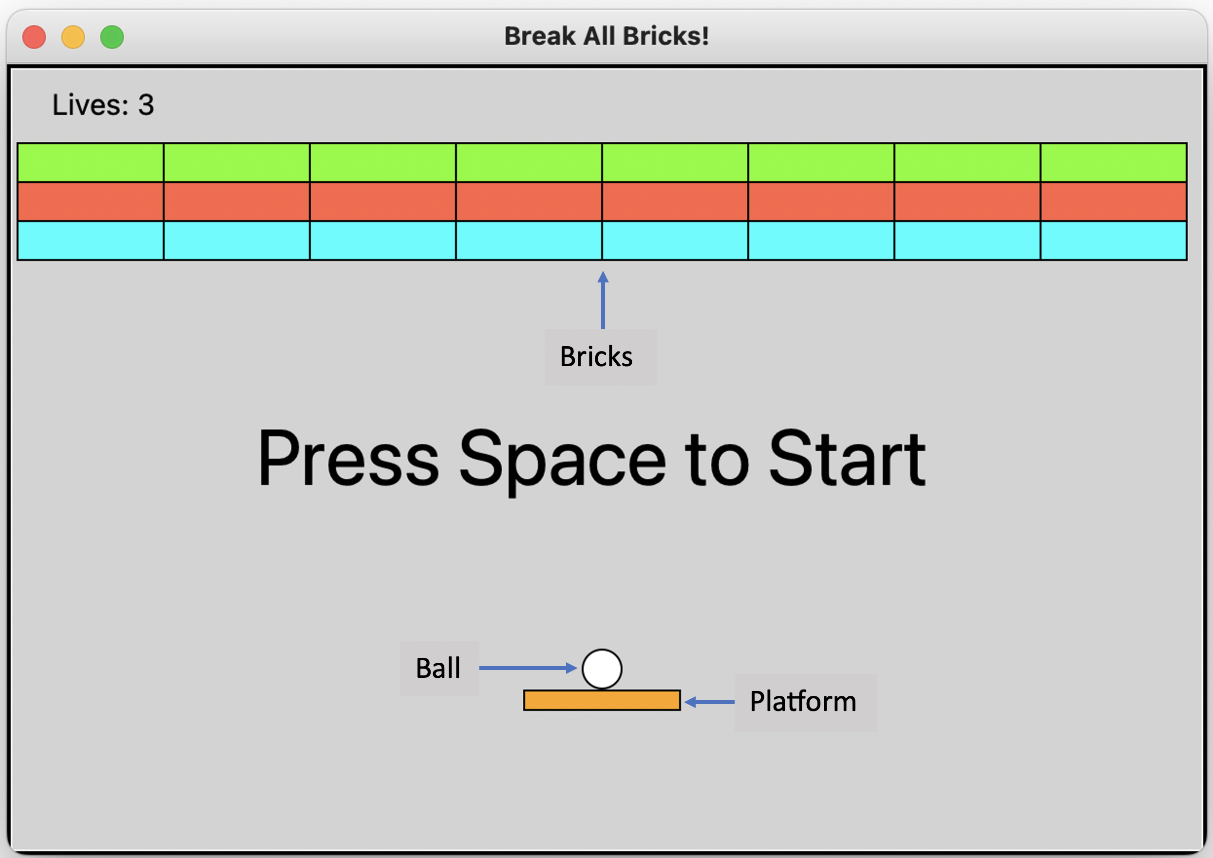
Parent Class
Class1 Brick_Breaker_Game
Attributes: canvas, item
Methods: get_position, move, delete
Child Class
Class2: Ball
Attributes: canvas, x , y
Methods: update, collide
Child Class
Class3: Paddle
Attributes: canvas, x , y
Methods: set_ball, move
Child Class
Class4: Brick
Attributes: canvas, x , y , hits
Methods: hit
Class4: Game
Attributes: master
Methods: setup_game, add_ball, add_brick, draw_text, update_lives_text, start_game, game_loop, check_collisions
# Brick Breaker Game.
# The tkinter package (“Tk interface”) is the standard Python interface
# to the Tcl/Tk GUI toolkit.
import tkinter as tk

class GameObject(object):
    # Attributes.
    def __init__(self, canvas, item):
        self.canvas = canvas
        self.item = item
    # Methods.
    def get_position(self):
        return self.canvas.coords(self.item)
    def move(self, x, y):
        self.canvas.move(self.item, x, y)
    def delete(self):
        self.canvas.delete(self.item)


class Ball(GameObject):
    # Attributes.
    def __init__(self, canvas, x, y):
        self.radius = 10
        self.direction = [1, -1]
        # Set the speed of the ball.
        self.speed = 4
        item = canvas.create_oval(x-self.radius, y-self.radius,
                                  x+self.radius, y+self.radius,
                                  fill="white")
        super(Ball, self).__init__(canvas, item)
    # Methods.
    def update(self):
        coords = self.get_position()
        width = self.canvas.winfo_width()
        if coords[0] <= 0 or coords[2] >= width:
            self.direction[0] *= -1
        if coords[1] <= 0:
            self.direction[1] *= -1
        x = self.direction[0] * self.speed
        y = self.direction[1] * self.speed
        self.move(x, y)
    def collide(self, game_objects):
        coords = self.get_position()
        x = (coords[0] + coords[2]) * 0.5
        if len(game_objects) > 1:
            self.direction[1] *= -1
        elif len(game_objects) == 1:
            game_object = game_objects[0]
            coords = game_object.get_position()
            if x > coords[2]:
                self.direction[0] = 1
            elif x < coords[0]:
                self.direction[0] = -1
            else:
                self.direction[1] *= -1
        for game_object in game_objects:
            if isinstance(game_object, Brick):
                game_object.hit()


class Paddle(GameObject):
    # Attributes.
    def __init__(self, canvas, x, y):
        self.width = 80
        self.height = 10
        self.ball = None
        item = canvas.create_rectangle(x - self.width / 2,
                                       y - self.height / 2,
                                       x + self.width / 2,
                                       y + self.height / 2,
                                       fill="Orange") # Paddle color.
        super(Paddle, self).__init__(canvas, item)
    # Methods.
    def set_ball(self, ball):
        self.ball = ball
    def move(self, offset):
        coords = self.get_position()
        width = self.canvas.winfo_width()
        if coords[0] + offset >= 0 and coords[2] + offset <= width:
            super(Paddle, self).move(offset, 0)
            if self.ball is not None:
                self.ball.move(offset, 0)


class Brick(GameObject):
    # Attributes.
    COLORS = {1: "Aqua", 2: "Tomato", 3: "LawnGreen"} # Brick colors.
    def __init__(self, canvas, x, y, hits):
        self.width = 75
        self.height = 20
        self.hits = hits
        color = Brick.COLORS[hits]
        item = canvas.create_rectangle(x - self.width / 2,
                                       y - self.height / 2,
                                       x + self.width / 2,
                                       y + self.height / 2,
                                       fill=color, tags='brick')
        super(Brick, self).__init__(canvas, item)
    # Methods.
    def hit(self):
        self.hits -= 1
        if self.hits == 0:
            self.delete()
        else:
            self.canvas.itemconfig(self.item,
                                   fill=Brick.COLORS[self.hits])


class Game(tk.Frame):
    # Attributes.
    def __init__(self, master):
        super(Game, self).__init__(master)
        self.lives = 3
        self.width = 610
        self.height = 400
        self.canvas = tk.Canvas(self, bg="LightGray", # Background color.
                                width=self.width,
                                height=self.height,)
        self.canvas.pack()
        self.pack()

        self.items = {}
        self.ball = None
        self.paddle = Paddle(self.canvas, self.width/2, 326)
        self.items[self.paddle.item] = self.paddle
        # Adding brick with different hit capacities: 3, 2 and 1.
        for x in range(5, self.width - 5, 75):
            self.add_brick(x + 37.5, 50, 3)
            self.add_brick(x + 37.5, 70, 2)
            self.add_brick(x + 37.5, 90, 1)

        self.hud = None
        self.setup_game()
        self.canvas.focus_set()
        self.canvas.bind("<Left>",
                         lambda _: self.paddle.move(-10))
        self.canvas.bind("<Right>",
                         lambda _: self.paddle.move(10))

    def setup_game(self):
           self.add_ball()
           self.update_lives_text()
           self.text = self.draw_text(300, 200,
                                      "Press Space to Start")
           self.canvas.bind("<space>", lambda _: self.start_game())

    def add_ball(self):
        if self.ball is not None:
            self.ball.delete()
        paddle_coords = self.paddle.get_position()
        x = (paddle_coords[0] + paddle_coords[2]) * 0.5
        self.ball = Ball(self.canvas, x, 310)
        self.paddle.set_ball(self.ball)

    def add_brick(self, x, y, hits):
        brick = Brick(self.canvas, x, y, hits)
        self.items[brick.item] = brick

    def draw_text(self, x, y, text, size="40"):
        font = ("Forte", size)
        return self.canvas.create_text(x, y, text=text,
                                       font=font)

    def update_lives_text(self):
        text = "Lives: %s" % self.lives
        if self.hud is None:
            self.hud = self.draw_text(50, 20, text, 15)
        else:
            self.canvas.itemconfig(self.hud, text=text)

    def start_game(self):
        self.canvas.unbind("<space>")
        self.canvas.delete(self.text)
        self.paddle.ball = None
        self.game_loop()

    def game_loop(self):
        self.check_collisions()
        num_bricks = len(self.canvas.find_withtag("brick"))
        if num_bricks == 0:
            self.ball.speed = None
            self.draw_text(300, 200, "WINNER - You broke all of the bricks!")
        elif self.ball.get_position()[3] >= self.height:
            self.ball.speed = None
            self.lives -= 1
            if self.lives < 0:
                self.draw_text(300, 200, "Sorry - You Lose! Game Over!")
            else:
                self.after(1000, self.setup_game)
        else:
            self.ball.update()
            self.after(50, self.game_loop)

    def check_collisions(self):
        ball_coords = self.ball.get_position()
        items = self.canvas.find_overlapping(*ball_coords)
        objects = [self.items[x] for x in items if x in self.items]
        self.ball.collide(objects)

if __name__ == "__main__":
    root = tk.Tk()
    root.title("Break All Bricks!")
    game = Game(root)
    game.mainloop()
© Stephen Lynch 2023-present.