Python for A-Level Mathematics and Beyond
© Professor Stephen Lynch NTF FIMA SFHEA
Homepage: https://www.lboro.ac.uk/departments/compsci/staff/stephen-lynch/

Introduction
This notebook lists examples of simple Python commands and programs that can be used to help with the understanding of the new A-Level syllabus. Teachers can use the examples to help with teaching or to make up examples and exercises. Pupils can use Python to check their answers and learn programming to help with employability. As you will discover, Python can help with all of the MEI schemes of work listed in the table above.
This is a Jupyter notebook launched from within the Anaconda data science platform. Anaconda can be downloaded here:
Python is an open-source programming language used extensively around the world. It is also vital for carrying out Scientific Computation!
To execute commands in Jupyter, either Run the cell or hit SHIFT + ENTER.
More information on why you should learn Python is given here: Python for A-Level Maths, Undergraduate Maths and Employability
Alternatively, you can perform cloud computing using Google Colab:
https://colab.research.google.com/
You will need a Google account to perform cloud computing.
1. Surds and Indices
From the sympy module import sqrt and simplify.
(i) Simplify $(2 + 2 \sqrt{2})(-\sqrt{2} + 4)$.
(ii) Simplify $\frac{6}{5 \sqrt{2}}$ and $\frac{1}{2-\sqrt{5}}$
(iii) Expand $(2-3 \sqrt{5})^{10}$. Do not do this by hand!
# Load functions from the SYMbolic PYthon module.
from sympy import sqrt, simplify
simplify((2 + 2 * sqrt(2))*(-sqrt(2) + 4))
print(simplify(6 / (5 * sqrt(2))))

print(simplify(1 / (2 - sqrt(5))))
3*sqrt(2)/5
-sqrt(5) - 2
simplify((2 - 3 * sqrt(5))**10)
Find, to 3 significant figures, the value of $x$ for which $8^x=0.8$.
from sympy import Symbol, solve
x = Symbol("x")
sol = solve(8**x - 0.8, x)
# Zero-based indexing in Python: sol[0] is the first solution.
# The other two roots are complex.
# Format the solution.
print("The real solution is {:0.3g},".format(sol[0]), "to 3 sig. figs.")
The real solution is -0.107, to 3 sig. figs.
2. Quadratic Functions
From sympy import solve and Symbol. Import numpy and matplotlib.
(i) Determine the roots of the equation: $x^2+3x-5=0$.
(ii) Plot the quadratic function: $y=x^2+3x-5$.
from sympy import solve, Symbol
x = Symbol("x")
solve(x**2 + 3 * x - 5, x)
[-3/2 + sqrt(29)/2, -sqrt(29)/2 - 3/2]
# Use the alias np instead of numpy (NUMerical PYthon).
# Use the alias plt for matplotlib.pyplot.
import numpy as np
import matplotlib.pyplot as plt
# x ranges from -8 to 5 in 100 intervals.
x = np.linspace(-8, 5, 100)
plt.plot(x, x**2 + 3 * x - 5)
plt.xlabel("x")
plt.ylabel("y")
# Show the plot.
plt.show()

3. Equations and Inequalities
(i) Solve the simultaneous equations: $2x+y=4, x^2-y=4$.
(ii) Solve the inequality $x^2-4x+1 \geq x-3$.
from sympy import solve, symbols
x, y = symbols('x, y')
solve((2 * x + y - 4, x**2 - y - 4), x, y)
[(-4, 12), (2, 0)]
solve(x**2 - 4 * x + 1 >= x - 3, x)
4. Coordinate Geometry
Plot a tangent to a circle.
(i) Plot the circle $x^2+y^2-2x-2y-23=0$.
(ii) Plot the line $4x-3y-26=0$.
import numpy as np
import matplotlib.pyplot as plt
# Set the dimensions of the figure.
fig = plt.figure(figsize = (6, 6))
x, y = np.mgrid[-6:8:100j,-6:8:100j]
z = x**2 + y**2 - 2 * x - 2 * y
# You can plot multiple contours if desired.
plt.contour(x, y, z, levels = [23])
x = np.linspace(2, 8, 100)
y = (4 * x - 26) / 3
plt.plot(x, y)
plt.xlabel('x')
plt.ylabel('y')
plt.show()

5. Trigonometry
Plot the trigonometric functions $y=2\sin(3t)$ and $y=3\cos(2t-\pi)$ on one graph.
import numpy as np
import matplotlib.pyplot as plt
t = np.linspace(-2 * np.pi, 2 * np.pi, 100)
# LaTeX code in labels.
plt.plot(t, 2 * np.sin(3 * t), label = '$2\sin(3t)$')
plt.plot(t, 3 * np.cos(2 * t - np.pi), label ='$3\cos(2t-\pi)$')
legend = plt.legend()
plt.show()

6. Polynomials
(i) Factorize $2x^4-x^3-4x^2-5x-12$.
(ii) Expand $\left(x^2-x+1\right)\left(x^3-x^2+x\right)$.
from sympy import expand, factor, Symbol
x = Symbol('x')
p1 = factor(2 * x**4 - x**3 - 4 * x**2 - 5 * x - 12)
p2 = expand((x**2 - x + 1) * (x**3 - x**2 + x))
print(p1)
print(p2)
(2*x + 3)*(x**3 - 2*x**2 + x - 4)
x**5 - 2*x**4 + 3*x**3 - 2*x**2 + x
7. Graphs and Transformations
Plot the trigonometric functions $y_1=sin(t)$ and $y_2=2+2sin(3t+\pi)$ on one graph.
import numpy as np
import matplotlib.pyplot as plt
t = np.linspace(-2 * np.pi, 2 * np.pi, 100)
plt.plot(t, np.sin(t), t, 2 + 2 * np.sin(3 * t + np.pi))
plt.xlabel('t')
# LaTeX code in ylabel.
plt.ylabel('$y_1, y_2$')
plt.show()

Animation
Produce an animation of the sine wave, $y=\sin(\omega t)$, for $0 \leq \omega \leq 10$. In this case, the frequency of the sine wave is changing. A slider appears under the figure. You can set the animation to Reflect to see how the curve changes as a parameter increases and decreases.
import numpy as np
from matplotlib import pyplot as plt
from matplotlib import animation

fig = plt.figure()
ax = plt.axes(xlim=(0, 2),ylim=(-2, 2))
line, = ax.plot([],[],lw=2)
plt.xlabel('time')
plt.ylabel('sin($\omega$t)')
plt.close()

def init():
    line.set_data([],[])
    return line,

# The function to animate.
# frames = 101, so 0 <= i <= 100.
def animate(i):
    x = np.linspace(0, 2, 1000)
    y = np.sin((0.1 * i * x))
    line.set_data(x, y)
    return line,

# Note: blit=True means only re-draw the parts that have changed.
anim = animation.FuncAnimation(fig, animate, init_func=init, \
                               frames=101, interval=200, blit=False)

# The code to produce an animation in html.
from IPython.display import HTML
HTML(anim.to_jshtml())
Interactive plot
The amplitude $A$ varies $0 \leq A \leq 5$, in steps of $0.2$, the frequency $B$ varies $0 \leq B \le 2\pi$, the phase $C$ varies $0 \leq C \leq 2\pi$ and the vertical shift $D$ varies $-3 \leq D \leq 3$, in steps of $0.5$.
You will get an interactive plot if you run the cell below.
# Interactive plots with Python.
from __future__ import print_function
from ipywidgets import interact, interactive, fixed, interact_manual
import ipywidgets as widgets

%matplotlib inline
from ipywidgets import interactive
import matplotlib.pyplot as plt
import numpy as np

# Interactive plot showing amplitude, frequency, phase and vertical shift.

def f(A, B, C, D):
    plt.figure(2)
    x = np.linspace(-10, 10, num=1000)
    plt.plot(x, A * np.sin(B * (x + C)) + D)
    plt.ylim(-8, 8)
    plt.show()

interactive_plot = interactive(f, A = (0, 5, 0.2), B = (0, 2 * np.pi), \
                               C = (0, 2 * np.pi),  D = (-3, 3, 0.5))
output = interactive_plot.children[-1]
output.layout.height = '350px'
interactive_plot
interactive(children=(FloatSlider(value=2.0, description='A', max=5.0, step=0.2), FloatSlider(value=3.14159265…
8. The Binomial Expansion
(i) Expand $(1-2x)^6$.
(ii) Plot the graph of $B(n)=\left(1+\frac{1}{n} \right)^n$.
from sympy import expand, Symbol
import numpy as np
import matplotlib.pyplot as plt
x = Symbol('x')
p1 = expand((1 - 2 * x)**6)
print("(1 - 2 * x)**6 =", p1)
n = np.linspace(1, 100, 100)
plt.plot((1 + 1/ n)**n)
plt.xlabel('n')
plt.ylabel('B(n)')
plt.show()
(1 - 2 * x)**6 = 64*x**6 - 192*x**5 + 240*x**4 - 160*x**3 + 60*x**2 - 12*x + 1

9. Differentiation
Determine:
(i) the first derivative of $x^3 + 3x^2 - 7x + 5$;
(ii) the second derivative of $4x^3 - 3x^4$.
from sympy import diff, Symbol
x = Symbol('x')
d1 = diff(x**3 + 3 * x**2 - 7 * x + 5, x)
print(d1)
d2 = diff(4 * x**3 - 3 * x**4, x, 2)
print(d2)
3*x**2 + 6*x - 7
12*x*(2 - 3*x)
10. Integration
Determine:
(i) the indefinite integral $I_1 = \int x^4+3x^3-8 dx$;
(ii) the definite integral $I_2 = \int_{x=0}^{\pi} sin(x)cos(x) dx$.
from sympy import *
x = Symbol('x')
i1 = integrate(x**4 + 3 * x**3 - 8)
print('I_1 =', i1, "+ c")
i2 = integrate(sin(x) * cos(x), (x, 0, pi))
print('I_2 =',i2)
I_1 = x**5/5 + 3*x**4/4 - 8*x + c
I_2 = 0
11. Vectors
Given that $\underline{u}=(1, 3)$ and $\underline{v}=(3, -5)$, determine:
(i) $\underline{w}=2\underline{u}+3\underline{v}$;
(ii) the distance between $\underline{u}$ and $\underline{v}$, $d=\| \underline{u}-\underline{v} \|$.
The length of the vector $\underline{u}=\left( u_1,u_2 \right)$, or the norm of $\underline{u}$, is defined to be $\|\underline{u} \|=\sqrt{u_1^2+u_2^2}$.
import numpy as np
u = np.array([1, 3])
v = np.array([3, -5])
w = 2 * u + 3 * v
print("w =", w)
d = np.linalg.norm(u - v)
print("d =", d)
w = [11 -9]
d = 8.246211251235321
12. Exponentials and Logarithms
(i) Determine $e^{10}$ and $\log_{10}(22026.4658)$.
(ii) Plot the graph, $x=1-e^{-t}$.
(iii) Solve the equation $7^{x-3}=4$.
import numpy as np
import matplotlib.pyplot as plt
exp10 = np.exp(10)
print("exp(10) =", exp10)
log10 = np.log(22026.4658)
print("log(22026.4658) =", log10)
t = np.linspace(0, 10, 100)
x = 1 - np.exp(- t)
plt.plot(t, x)
plt.xlabel('t')
plt.ylabel('x(t)')
plt.show()

from sympy import Symbol
x = Symbol('x')
sol = solve(7**(x-3) - 4)
print('The solution to', '7**{x-3}=4 is,', sol)
exp(10) = 22026.465794806718
log(22026.4658) = 10.000000000235774

The solution to 7**{x-3}=4 is, [log(1372)/log(7)]
13. Data Collection
(i) Select 10 random numbers from a list of the first 25 natural numbers.
(ii) Select 10 randon numbers from a list of the first 100 even natural numbers.
import math, random, statistics
a = list(range(1, 26))
data1 = random.sample(a, 10)
print("data1 =", data1)
b = list(range(2, 102, 2))
data2 = random.sample(b, 10)
print("data2 =", data2)
data1 = [25, 9, 12, 2, 23, 18, 24, 13, 22, 1]
data2 = [20, 44, 90, 4, 68, 62, 46, 34, 14, 70]
14. Data Processing
Determine the mean, median, mode, variance and standard deviation of the data set:
[43, 39, 41, 48, 49, 56, 55, 44, 44, 32, 20, 44, 48, 2, 98].
import statistics as stats
data1 = [43, 39, 41, 48, 49, 56, 55, 44, 44, 32, 20, 44, 48, 2, 98]
mean_data1 = stats.mean(data1)
print("mean_data1 =", mean_data1)
median_data1 = stats.median(data1)
print("median_data1 =", median_data1)
mode_data1 = stats.mode(data1)
print("mode_data1 =", mode_data1)
var_data1 = stats.variance(data1)
print("var_data1 =", var_data1)
stdev_data1 = stats.stdev(data1)
print("stdev_data1 =", stdev_data1)
mean_data1 = 44.2
median_data1 = 44
mode_data1 = 44
var_data1 = 411.1714285714286
stdev_data1 = 20.277362465849166
15. Probability
Plot a Venn diagram for the following data. The following shows the results of a survey on the types of exercises taken by a group of 100 pupils: 65 run, 48 swim, 60 cycle, 40 run and swim, 30 swim and cycle, 35 run and cycle and 25 do all 3. Draw a Venn diagram to represent these data.
Let A denote the set of pupils who run, B represent the set of pupils who swim and C contain the set of pupils who cycle.
!pip install matplotlib-venn
Requirement already satisfied: matplotlib-venn in /Users/admin/anaconda3/lib/python3.11/site-packages (1.0.0)
Requirement already satisfied: matplotlib in /Users/admin/anaconda3/lib/python3.11/site-packages (from matplotlib-venn) (3.7.2)
Requirement already satisfied: numpy in /Users/admin/anaconda3/lib/python3.11/site-packages (from matplotlib-venn) (1.24.3)
Requirement already satisfied: scipy in /Users/admin/anaconda3/lib/python3.11/site-packages (from matplotlib-venn) (1.11.1)
Requirement already satisfied: contourpy>=1.0.1 in /Users/admin/anaconda3/lib/python3.11/site-packages (from matplotlib->matplotlib-venn) (1.0.5)
Requirement already satisfied: cycler>=0.10 in /Users/admin/anaconda3/lib/python3.11/site-packages (from matplotlib->matplotlib-venn) (0.11.0)
Requirement already satisfied: fonttools>=4.22.0 in /Users/admin/anaconda3/lib/python3.11/site-packages (from matplotlib->matplotlib-venn) (4.25.0)
Requirement already satisfied: kiwisolver>=1.0.1 in /Users/admin/anaconda3/lib/python3.11/site-packages (from matplotlib->matplotlib-venn) (1.4.4)
Requirement already satisfied: packaging>=20.0 in /Users/admin/anaconda3/lib/python3.11/site-packages (from matplotlib->matplotlib-venn) (23.1)
Requirement already satisfied: pillow>=6.2.0 in /Users/admin/anaconda3/lib/python3.11/site-packages (from matplotlib->matplotlib-venn) (9.4.0)
Requirement already satisfied: pyparsing<3.1,>=2.3.1 in /Users/admin/anaconda3/lib/python3.11/site-packages (from matplotlib->matplotlib-venn) (3.0.9)
Requirement already satisfied: python-dateutil>=2.7 in /Users/admin/anaconda3/lib/python3.11/site-packages (from matplotlib->matplotlib-venn) (2.8.2)
Requirement already satisfied: six>=1.5 in /Users/admin/anaconda3/lib/python3.11/site-packages (from python-dateutil>=2.7->matplotlib->matplotlib-venn) (1.16.0)
# Venn Diagram.
# Install the matplotlib-venn library on to your computer.
# In the Terminal type: conda install -c conda-forge matplotlib-venn
# Alternatively, run the code in Google Colab.
import matplotlib.pyplot as plt
import numpy as np
from matplotlib_venn import venn3
fig, ax = plt.subplots(facecolor='lightgray')
ax.axis([0, 1, 0, 1])
v = venn3(subsets = (15, 3, 15, 20, 10, 5, 25))
ax.text(1, 1, "7")
plt.show()

16. The Binomial Distribution
The binomial distribution is an example of a discrete probability distribution function.
Given $X \sim B(n,p)$, then $P(X=r)={n \choose r}p^r(1-p)^{n-r}$,
where $X$ is a binomial random variable, and $p$ is the probability of $r$ success from $n$ independent trials. Note that (i) the expectation, $E(X)=np$; (ii) the variance, $\mathrm{var}(X)=np(1-p)$; and (iii) the standard deviation, $\mathrm{std}=\sqrt{np(1-p)}$.
Example: Manufacturers of a bag of sweets claim that there is a 90% chance that the bag contains some toffees. If 20 bags are chosen, what is the probability that:
(a) All bags contain toffees?
(b) More than 18 bags contain toffees?
from scipy.stats import binom
import matplotlib.pyplot as plt
n , p = 20 , 0.9
r_values = list(range(n+1))
dist = [binom.pmf(r , n , p) for r in r_values]
plt.bar(r_values , dist)
plt.show()
print('Mean = ', binom.mean(n = 20 , p = 0.9))
print('Variance = ', binom.var(n = 20 , p = 0.9))
print('Standard Deviation = ', binom.std(n = 20 , p = 0.9))

PXis20 = binom.pmf(20, n, p)      # Probability mass function.
print('P(X=20)=' , PXis20)
PXGT18 = 1 - binom.cdf(18, n, p)  # Cumulative distribution function.
print('P(X>18)=' , PXGT18 )       # P(X>18)=1-P(X<=18).

Mean =  18.0
Variance =  1.7999999999999996
Standard Deviation =  1.3416407864998736
P(X=20)= 0.12157665459056935
P(X>18)= 0.3917469981251679
17. Hypothesis Testing
Example: The probability of a patient recovering from illness after taking a drug is thought to be 0.85. From a trial of 30 patients with the illness, 29 recovered after taking the drug. Test, at the 10% level, whether the probability is different to 0.85.
So, $H_0=0.85$,
$H_1 \neq 0.85$. (Two-tail test)
The program below gives $P(X \geq 29)=0.0480<0.05$.
Therefore, the result is significant and so we reject $H_0$. There is evidence to suggest that the probability of recovery from the illness after taking the drug is different to 0.85.
from scipy.stats import binom
import matplotlib.pyplot as plt
n , p = 30 , 0.85
r_values = list(range(n+1))
dist = [binom.pmf(r , n , p) for r in r_values]
plt.bar(r_values , dist)
plt.show()
print('Mean = ', binom.mean(n = 30 , p = 0.85))
print('Variance = ', binom.var(n = 30 , p = 0.85))
print('Standard Deviation = ', binom.std(n = 30 , p = 0.85))
PXGTE29 = 1 - binom.cdf(28, n, p)  # Cumulative distribution function.
print('P(X>=29)=' , PXGTE29 )      # P(X>=29)=1-P(X<=28).

Mean =  25.5
Variance =  3.8250000000000006
Standard Deviation =  1.9557607215607948
P(X>=29)= 0.04802889862602788
18. Kinematics
Plot a velocity time graph.
import matplotlib.pyplot as plt
xs = [0, 3, 9, 15]
ys = [14, 8, 8, -4]
plt.axis([0, 15, -4, 14])
plt.plot(xs, ys)
plt.xlabel('time(s)')
plt.ylabel('velocity (m/s)')
plt.show()

19. Forces and Newton's Laws
Plot a forces diagram.
import matplotlib.pyplot as plt
ax = plt.axes()
plt.axis([-2, 2, -2, 2])
ax.arrow(0,0,0,1.5,head_width=0.05,head_length=0.1,fc='k',ec='k')
ax.arrow(0,0,1.5,0,head_width=0.05,head_length=0.1,fc='r',ec='r')
ax.arrow(0,0,-1.5,-1.5,head_width=0.05,head_length=0.1,fc='b',ec='b')
plt.text(0.1,1.5,'$F_1$',fontsize=15)
plt.text(1.5,0.1,'$F_2$',{'color':'red','fontsize':15})
plt.text(-1.5,-1.2,'$F_3$',{'color':'blue','fontsize':15})
plt.show()

20. Variable Acceleration
Plot a velocity-time graph.
import numpy as np
import matplotlib.pyplot as plt
pts = np.array([0,1,2,3,3,3,2,1,3,6,10,15])
fig = plt.figure()
plt.plot(pts)
plt.xlabel('time(s)')
plt.ylabel('velocity (m/s)')
plt.show()

21. Proof
There are research groups around the world who are using AI for mathematical proof! There is a reference in the book.
(i) For the natural numbers up to 100, investigate when $2n^2$, is close to a perfect square.
This will give a good approximation to $\sqrt{2}$. Can you explain why?
(ii) Prove by elimination, that there is only one solution to the equation:
$m^2-17n^2=1$, where $m$ and $n$ are natural numbers and $1 \leq m \le 500$, $1 \leq n \le 500$.
Print the unique values of $m$ and $n$.
import numpy as np
for n in range(1, 101):
    num1 = np.sqrt(2 * n**2)
    num2 = int(np.round(np.sqrt(2 * n**2)))
    if abs(num1 - num2) < 0.01:
        print(num2, 'divided by', n, 'is approximately sqrt(2)')
99 divided by 70 is approximately sqrt(2)
140 divided by 99 is approximately sqrt(2)
# An example of a program with for loops and if statements.
# The final value, 501, is not included in range in Python.
for m in range(1, 501):
    for n in range(1, 501):
        if m**2 - 17 * n**2 == 1:        # Note the Boolean ==.
            print('The unique solution is, m =',m, 'and n =',n)
The unique solution is, m = 33 and n = 8
22. Trigonometry
By plotting curves, show that:
(i) $\sin(t) \approx t$, near $t=0$;
(ii) $\cos(t) \approx 1 - \frac{t^2}{2}$, near $t=0$.
import numpy as np
import matplotlib.pyplot as plt
plt.figure(1)
plt.subplot(121)
t = np.linspace(- 2, 2, 100)
plt.plot(t, np.sin(t), t, t)
plt.xlabel('t')
plt.ylabel('f(t)')
plt.subplot(122)
t = np.linspace(- 2, 2, 100)
plt.plot(t, np.cos(t), t, 1 - t**2 / 2)
plt.xlabel('t')
plt.ylabel('f(t)')
plt.subplots_adjust(wspace=1)
plt.show()

23. Sequences and Series
Given that, for an arithemtic series:
$a_n=a+(n-1)d$
$S_n=\sum_{i=1}^{n} \, a+(n-1)d$.
Determine:
(i) the term $a_{20}$,
(ii) the sum $S_{20}$,
when $a=3$ and $d=6$.
def nthterm(a, d, n):
    term = a + (n - 1) * d
    return(term)
def sumofAP(a, d, n):
    sum, i = 0, 0
    while i < n:
        sum += a
        a = a + d
        i += 1             # i = i + 1.
    return sum
a, d, n = 3, 6, 20
print('The', n, 'th', 'term is', nthterm(a, d, n))
print('The sum of the', n, 'terms is', sumofAP(a, d, n))
The 20 th term is 117
The sum of the 20 terms is 1200
from sympy import expand, Symbol
x = Symbol('x')
def f(x):
    return(1 - x**2)
print('f(x) = ', f(x))
print('f(2) = ', f(2))
print('f(f(x)) = ', expand(f(f(x))))
f(x) =  1 - x**2
f(2) =  -3
f(f(x)) =  -x**4 + 2*x**2
25. Differentiation
Given that, $f(x)=\frac{x}{\sqrt{2x-1}}$, determine $\left. \frac{df}{dx} \right|_{x=5}$.
from sympy import diff, sqrt, Symbol
x = Symbol('x')
df = diff(x / sqrt(2 * x - 1), x)
print('df/dx = ', df)
dfx = df.subs(x, 5)
print('Gradient at x = 5 is', dfx)
df/dx =  -x/(2*x - 1)**(3/2) + 1/sqrt(2*x - 1)
Gradient at x = 5 is 4/27
26. Trigonometric Functions
Plot the curve $\sec(t)=\frac{1}{\cos(t)}$.
import numpy as np
import matplotlib.pyplot as plt
t = np.linspace(- 2 * np.pi, 2 * np.pi, 1000)
plt.axis([-2 * np.pi, 2 * np.pi, -10, 10])
plt.plot(t, 1 / np.cos(t))
plt.xlabel('t')
plt.ylabel('sec(t)')
plt.show()

Solve the trigonometric equation: $2\cos(x) + 5\sin(x)=3$.
from sympy import *
x = Symbol('x')
solve(2 * cos(x) + 5 * sin(x) - 3)
[2*atan(1 - 2*sqrt(5)/5), 2*atan(2*sqrt(5)/5 + 1)]
27. Algebra
Split $\frac{2x+3}{(x-2)(x-3)(x-4)}$ into partial fractions.
from sympy import *
x = Symbol('x')
apart((2 * x + 3)/((x - 2) * (x - 3) * (x - 4)))
(i) Determine the $O(x^{10})$ Taylor series expansion of $\frac{1}{2-x}$, at $x=0$.
(ii) By plotting curves, show that $\frac{1}{2-x} \approx \frac{1}{2}+\frac{x}{4}+\frac{x^2}{8}$, at $x=0$.
import numpy as np
import matplotlib.pyplot as plt
from sympy import series, Symbol
x = Symbol('x')
Taylor_series = series(1 / (2 - x), x, 0 , 10)
print('The Taylor series of 1/(2-x) is ', Taylor_series)
x = np.linspace(-1.5, 1.5, 100)
plt.axis([-1.5, 1.5, 0, 3])
plt.plot(x, 1/(2 - x), label = '1/(2-x)')
plt.plot(x, 1/2 + x/4 + x**2/8, label = 'Taylor series')
legend = plt.legend()
plt.xlabel('x')
plt.show()
The Taylor series of 1/(2-x) is 1/2 + x/4 + x**2/8 + x**3/16 + x**4/32 + x**5/64 + x**6/128 + x**7/256 + x**8/512 + x**9/1024 + O(x**10)

28. Trigonometric Identities
Show that the curves $f(t)=\sqrt{2}\cos(t)+\sin(t)$, and $g(t)=\sqrt{3}\cos(t-\alpha)$, are equivalent, where $\alpha=\tan^{-1}\left( {\frac{1}{\sqrt{2}}} \right)$.
import numpy as np
from sympy import sqrt
from math import atan
import matplotlib.pyplot as plt
alpha = atan(1/sqrt(2))
t = np.linspace(- 2 * np.pi, 2 * np.pi, 100)
plt.plot(t, sqrt(2) * np.cos(t) + np.sin(t), 'r-',linewidth = 10)
plt.plot(t, sqrt(3) * np.cos(t - alpha), 'b-', linewidth = 4)
plt.xlabel('t')
plt.ylabel('f(t)')
plt.show()

29. Further Differentiation
Differentiate:
(i) $f(x)=3x^2e^{-3x}$;
(ii) $g(x)=\frac{3\sin(x)}{\ln(7x)}$;
(iii) $h(x)=\frac{xe^{-2x}\cos(x)}{(x+1)\sin(x)}$.
from sympy import diff, exp, log, sin, Symbol
x = Symbol('x')
print('df = ', diff(3 * x**2 * exp(- 3 * x), x))
print('dg = ', diff((3*sin(x))/log(7*x)))
print('dh =', diff((x*exp(-2*x)*cos(x)) / ((x+1)*sin(x))))
df =  -9*x**2*exp(-3*x) + 6*x*exp(-3*x)
dg =  3*cos(x)/log(7*x) - 3*sin(x)/(x*log(7*x)**2)
dh = -x*exp(-2*x)/(x + 1) - 2*x*exp(-2*x)*cos(x)/((x + 1)*sin(x)) - x*exp(-2*x)*cos(x)**2/((x + 1)*sin(x)**2) - x*exp(-2*x)*cos(x)/((x + 1)**2*sin(x)) + exp(-2*x)*cos(x)/((x + 1)*sin(x))
from sympy import cos, integrate, Symbol
x = Symbol('x')
I_1 = integrate(x**2 * cos(x**3), x)
print('I_1=',I_1, '+ c')
I_2 = integrate(x * cos(4 * x), x)
print('I_2=',I_2, '+ k')
I_1= sin(x**3)/3 + c
I_2= x*sin(4*x)/4 + cos(4*x)/16 + k
31. Parametric Equations
(i) Plot the parametric curve, $x(t)=1-\cos(t), y(t)=\sin(2t)$, for $0 \leq t \leq 2 \pi$.
(ii) Given the parametric equations: $x(t)=\sqrt{3}\sin(2t), y(t)=4\cos^2(t), 0 \leq t \leq \pi$, show that $\frac{dy}{dx}=k(\sqrt{3}\tan(2t)$, and determine $k$.
(iii) Plot the parametric curve, $x(t)=2\cos(2t), y(t)=6\sin(t), 0 \leq t \leq \frac{\pi}{2}$, and determine the area under the curve for $-2 \leq x \leq 2$.
(i) Use numpy and matplotlib to plot the parametric curve.
import numpy as np
import matplotlib.pyplot as plt
t = np.linspace(0, 2 * np.pi, 100)
x = 1 - np.cos(t)
y = np.sin(2 * t)
plt.plot(x, y)
plt.xlabel('x')
plt.ylabel('y')
plt.show()

(ii) Now, $\frac{dy}{dx}=\frac{\frac{dy}{dt}}{\frac{dx}{dt}}$. From the computation below, $k=-\frac{2}{3}$.
from sympy import *
t = symbols("t")
x = sqrt(3) * sin(2 * t)
y = 4 * cos(t)**2
dydt = diff(y , t) / diff(x , t)
trigsimp(dydt)
(iii) Plot the parametric curve.
import numpy as np
import matplotlib.pyplot as plt
t = np.linspace(0, np.pi / 2, 100)
x = 2 * np.cos(2 * t)
y = 6 * np.sin(t)
plt.plot(x, y)
plt.xlabel("x")
plt.ylabel("y")
plt.show()

Now, Area $=\int y dx = \int y(t) \frac{dx(t)}{dt} dt$.
from sympy import *
t = symbols("t")
x = 2 * cos(2 * t)
y = 6 * sin(t)
Area = integrate(y * diff(x , t) , (t , pi / 2 , 0))
print("Area = " , Area , "units squared")
Area = 16 units squared
32. Vectors
Given that $\underline{u}=(1,-1,4)$ and $\underline{v}=(2,-1,9)$, determine:
(i) $5\underline{u}-6\underline{v}$;
(ii) the distance between $\underline{u}$ and $\underline{v}$, $d=\| \underline{u}-\underline{v} \|$.
(iii) the angle, $\theta$, say, between $\underline{u}$ and $\underline{v}$.
Recall that $\cos{\theta}=\frac{\underline{u}.\underline{v}}{\|\underline{u} \| \|\underline{v} \|}$.
import numpy as np
from math import acos
u = np.array([1, -1, 4])
v = np.array([2, -1, 9])
w = 5 * u - 6 * v
print("w =", w)
d = np.linalg.norm(u - v)
print("d =", d)
theta = acos(np.dot(u,v)/(np.linalg.norm(u) * np.linalg.norm(v)))
print('theta =', theta, 'radians')
w = [ -7   1 -34]
d = 5.0990195135927845
theta = 0.13245459846204063 radians
33. Differential Equations
(i) Plot the solution to the initial value problem, $\frac{dP}{dt}=P(1-0.01P)$, given that $P(0)=400$. This is a simple population model.
import numpy as np
from sympy import dsolve, Function, symbols
import matplotlib.pyplot as plt
P = Function('P')
t = symbols('t')
ODE = P(t).diff(t) - P(t) * (1 - 0.01 * P(t))
print('P(t) =', dsolve(ODE, ics = {P(0):400}))
t = np.linspace(0, 10, 100)
# Plot the solution to the ODE, P(t).
plt.plot(t, 100.0/(1.0  - 0.75*np.exp(-t)))
plt.xlabel('t')
plt.ylabel('P(t)')
plt.show()
P(t) = Eq(P(t), -100.0/(-1.0 + 0.75*exp(-t)))

(ii) A very simple epidemic model is described by the differential equations:
$\frac{dS}{dt}=-\frac{\beta S I}{N}, \quad \frac{dI}{dt}=\frac{\beta S I}{N} -\gamma I, \quad \frac{dR}{dt}=\gamma I,$
where $S(t)$ is the susceptible population, $I(t)$ is the infected population, $R(t)$ is the recovered-immune population, $N$ is the total population, $\beta$ is the contact rate of the disease and $\gamma$ is the mean recovery rate. Plot the solution curves for $S(t), I(t), R(t)$, given that $N=1000$, $S(0)=999$, $I(0)=1$, $R(0)=0$, $\beta=0.5$ and $\gamma=0.1$. This could be a simple model of the spread of flu in a school.
# SIR Epidemic model.
import numpy as np
import matplotlib.pyplot as plt
from scipy.integrate import odeint
# Set the parameters.
beta, gamma = 0.5, 0.1
S0, I0, R0, N = 999, 1, 0, 1000
tmax, n = 100, 1000
def SIR_Model(X, t, beta, gamma):
    S, I, R = X
    dS = - beta * S * I / N
    dI = beta * S * I / N - gamma * I
    dR = gamma * I
    return(dS, dI, dR)
t = np.linspace(0, tmax, n)
f = odeint(SIR_Model, (S0, I0, R0), t, args = (beta, gamma))
S, I, R = f.T
plt.figure(1)
plt.xlabel('time (days)')
plt.ylabel('Populations')
plt.title('Susceptible-Infected-Recovered (SIR) Epidemic Model')
plt.plot(t, S, label = 'S')
plt.plot(t, I, label = 'I')
plt.plot(t, R, label = 'R')
legend = plt.legend(loc = 'best')
plt.show()

34. Numerical Methods
Use the Newton-Raphson method to find the root of $x^3-0.9x^2+2=0$, starting with the point $x_0=2$. Give your answer to four decimal places. Recall that:
$x_{n+1}=x_n-\frac{f\left(x_n\right)}{f'(x_n)}$.
def fn(x):
    return x**3 - 0.9 * x**2 + 2
def dfn(x):
    return 3 * x**2 - 1.8 * x
def NewtonRaphson(x):
    i = 0
    h = fn(x) / dfn(x)
    while abs(h) >= 0.0001:
        h = fn(x) / dfn(x)
        x = x - h
        i += 1              # i = i + 1
        print('x(', i ,')', 'is {:6.4f}.'.format(x))
# Start at x( 0 ) = 2.
NewtonRaphson(2)
x( 1 ) is 1.2381.
x( 2 ) is 0.1756.
x( 3 ) is 9.0222.
x( 4 ) is 6.1131.
x( 5 ) is 4.1665.
x( 6 ) is 2.8496.
x( 7 ) is 1.9224.
x( 8 ) is 1.1648.
x( 9 ) is -0.0307.
x( 10 ) is -34.4718.
x( 11 ) is -22.8835.
x( 12 ) is -15.1594.
x( 13 ) is -10.0129.
x( 14 ) is -6.5872.
x( 15 ) is -4.3139.
x( 16 ) is -2.8196.
x( 17 ) is -1.8664.
x( 18 ) is -1.3134.
x( 19 ) is -1.0722.
x( 20 ) is -1.0225.
x( 21 ) is -1.0205.
x( 22 ) is -1.0205.
35. Probability
Generate some random data in Python and compare the histogram to a normal probability distribution function. Deremine the mean and standard deviation of the data.
from scipy import stats
import numpy as np
import matplotlib.pyplot as plt
data = 50 * np.random.rand() * np.random.normal(10, 10, 100) + 20
plt.hist(data, density = True)
xt = plt.xticks()[0]
xmin, xmax = min(xt), max(xt)
lnspc = np.linspace(xmin, xmax, len(data))
m, s = stats.norm.fit(data)
pdf_g = stats.norm.pdf(lnspc, m, s)
plt.plot(lnspc, pdf_g)
print('Mean =', m)
print('Standard Deviation =', s)
plt.show()
Mean = 255.18892252542196
Standard Deviation = 239.80908015336678

36. Probablility Distributions
The normal probability density function (PDF) is an example of a continuous PDF.
The general form of a normal distribution is:
$f(x)=\frac{1}{\sigma \sqrt{2 \pi}} e^{-\frac{1}{2} \left(\frac{x-\mu}{\sigma} \right)^2 }$,
where $\mu$ is the mean or expectation of the distribution, $\sigma^2$, is the variance, amd $\sigma$ is the standard deviation.
Example: Suppose that $X$ is normally distributed with a mean of 80 and a standard deviation of 4. So, $X \sim N(80, 16)$. Plot the bell curve and determine:
(a) $P(X<75)$; (b) $P(X>83)$; (c) $P(72<X<76)$.
import matplotlib.pyplot as plt
import numpy as np
import scipy.stats as stats
import math

mu , variance = 80 , 4**2
sigma = math.sqrt(variance)
x = np.linspace(mu - 3*sigma, mu + 3*sigma, 100)
plt.plot(x, stats.norm.pdf(x, mu, sigma))
plt.show()

sola = stats.norm.cdf(75, loc=mu, scale=sigma)
print('P(X<75)=', sola)

solb = 1 - stats.norm.cdf(83, loc=mu, scale=sigma)
print('P(X>83)=', solb)

solc = stats.norm.cdf(76, loc=mu, scale=sigma) - \
       stats.norm.cdf(72, loc=mu, scale=sigma)
print('P(72<X<76)=', solc)

P(X<75)= 0.10564977366685535
P(X>83)= 0.22662735237686826
P(72<X<76)= 0.13590512198327787
37. Hypothesis Testing
Example: The diameters of circular cardboard drinks packs produced by a certain machine are normally distributed with a mean of 9cm and standard deviation of 0.15cm. After the machine is serviced a random sample of 30 mats is selected and their diameters are measured to see if the mean diameter has altered.
The mean of the sample was 8.95cm. Test at the 5% level, whether there is significant evidence of a change in the mean diameter of mats produced by the machine.
Now, the null hypothesis is, $H_0: \mu=9$,
The alternative hypothesis is, $H_1: \mu \neq 9$. (Two-tailed test)
See below. Since $P(X<=8.95)=0.033945>0.025$, accept $H_0$.
There is not enough evidence to suggest there has been a change in the mean diamater of the mats.
import matplotlib.pyplot as plt
import numpy as np
import scipy.stats as stats
import math

mu , variance = 9 , 0.15**2 / 30
sigma = math.sqrt(variance)
x = np.linspace(mu - 3*sigma, mu + 3*sigma, 100)
plt.plot(x, stats.norm.pdf(x, mu, sigma))
plt.show()

sol = stats.norm.cdf(8.95, loc=mu, scale=sigma)
print('P(X<=8.95)=', sol)

P(X<=8.95)= 0.033944577430912545
38. Kinematics
Given that, $\underline{u}=2\underline{i}+9\underline{j} \, ms^{-1}$, $\underline{a}=-9.8\underline{j} \, ms^{-2}$, and $t=0.2s$, show that the distance travelled is $\underline{s}=0.4\underline{i}+1.604\underline{j} \, m$.
Recall that:
$\underline{v}=\underline{u}+\underline{a}t$;
$\underline{v}^2=\underline{u}^2+2\underline{a}\, \underline{s}$;
$\underline{s}=\underline{u}t+\frac{1}{2}\underline{a}t^2$;
$\underline{s}=(\underline{u}+\underline{v}) \frac{t}{2}$.
import numpy as np
u = np.array([2, 9])
a = np.array([0, -9.8])
t = 0.2
s = u * t + a * t**2 / 2
print('Distance travelled =', s, 'm')
Distance travelled = [0.4 1.604] m
39. Forces and Motion
Determine the resultant force given, $\underline{F_A}=-20 \underline{j}$ N and $\underline{F_B}=-16\underline{i}-16\underline{j}$ N.
import numpy as np
FAx = 0
FAy = -20
FBx = -16 * np.sin(np.radians(40.8))
FBy = -16 * np.cos(np.radians(40.8))
FR = np.array([FAx + FBx, FAy + FBy])
FR_norm = np.linalg.norm(FR)
FR_angle = np.degrees(np.arctan(FR[1] / FR[0]))
print("FR =", FR_norm, "N")
print("FR Angle =", FR_angle, "degrees.")
FR = 33.77094662009231 N
FR Angle = 71.96622155260425 degrees.
40. Moments
Given that, $F_1=5$N, $F_2=2$N, where would a force of $F_3=3$N need to be placed to balance the beam?
import matplotlib.pyplot as plt
ax = plt.axes()
plt.plot([-10, 10], [0, 0])
plt.axis([-11, 11, -10, 10])
plt.plot([0], marker = "^")
ax.arrow(-5, 0, 0, -4, head_width = 1, head_length = 1, fc = 'k', ec = 'k')
ax.arrow(2.5, 0, 0, -1, head_width = 1, head_length = 1, fc = 'r', ec = 'r')
plt.text(-7, -5, '$F_1$', fontsize = 15)
plt.text(0.5, -2, '$F_2$', {'color': 'red', 'fontsize':15})
plt.show()

41. Projectiles
Plot the trajectory of a ball thrown from the top of a cliff. The ball is thrown from the top of a cliff of height $10$ metres with velocity $\underline{u}=20\sqrt{3}\underline{i}+20\underline{j} \, ms^{-1}$. Use the equation:
$\underline{s}=\underline{u}t+\frac{1}{2}\underline{a}t^2$.
import numpy as np
import matplotlib.pyplot as plt
x0, y0, sy, g, dt, t = 0, 10, 0, 9.8, 0.01, 0
vx0 = 20 * np.sqrt(3)
vy0 = 20
while sy >= 0:
    sx = vx0 * t
    sy = vy0 * t - g * t**2 / 2 + y0
    t = t + dt
    plt.plot(sx, sy, 'r.')
plt.xlabel('Range')
plt.ylabel('Height')
plt.show()

42. Friction
Determine the acceleration of the particle up the slope, given that the coefficient of friction, $\mu$ say, is $\mu=\frac{1}{4}$.
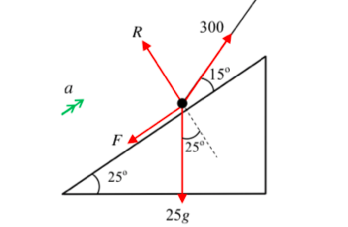
import numpy as np
# Resolve forces normal to slope.
R = 25 * 9.8 * np.cos(np.radians(25)) - 300 * np.sin(np.radians(15))
print("R =", R, "N")
# Since particle is moving.
F = (1 / 4) * R
print("F =", F, "N")
# Resolve forces parallel to slope.
a_num = 300 * np.cos(np.radians(15)) - F - 25 * 9.8 * np.sin(np.radians(25))
a = a_num / 25
print('a =', a, 'm/s/s.')
R = 144.39969429322304 N
F = 36.09992357330576 N
a = 6.005454007477733 m/s/s.
CRC Press (2024): https://www.routledge.com/A-Simple-Introduction-to-Python/Lynch/p/book/9781032750293
Support Material
GitHub Repository of Data Files and a Jupyter Solution notebook:
https://github.com/proflynch/A-Simple-Introduction-to-Python
Jupyter Solution notebook web page:
https://drstephenlynch.github.io/webpages/A-Simple-Introduction-to-Python-Solutions.html
CRC Press (2023): http://www.springer.com/us/book/9783319781440
Support Material
GitHub Repository of Python Files and Notebooks:
https://github.com/proflynch/CRC-Press/
Solutions to All Exercises:
Section 1: An Introduction to Python:
https://drstephenlynch.github.io/webpages/Solutions_Section_1.html
Section 2: Python for Scientific Computing:
https://drstephenlynch.github.io/webpages/Solutions_Section_2.html
Section 3: Artificial Intelligence:
https://drstephenlynch.github.io/webpages/Solutions_Section_3.html

Springer International Publishing (2018):
http://www.springer.com/us/book/9783319781440
Jupyter Notebook:
https://drstephenlynch.github.io/webpages/DSAP_Jupyter_Notebook.html
GitHub Files:
https://github.com/springer-math/dynamical-systems-with-applications-using-python